14 Appendix

14.1 Very introductory materials

About R: https://www.r-project.org/about.html
Getting started on R, (R documentation): https://cran.r-project.org/doc/manuals/r-release/R-intro.html
Getting started on R interactively, using the RStudio interface: https://swirlstats.com/

Here are two statistics texts, both of which have great introductory material on getting started with the R language.

http://users.miamioh.edu/fishert4/sta363/ (a great statistics text)
http://r-statistics.co/ (graphics and stats; has ads)

Arranging and summarizing data with dplyr: https://cran.r-project.org/web/packages/dplyr/vignettes/dplyr.html

R is a language. Use it every day, and you will learn it quickly.

14.2 Writing your own functions

One very cool thing in R is that you can write your own functions. Indeed it is the extensibility of R that makes it the home of cutting edge working, because edge cutters (i.e., leading scientists) can write code that we all can use. People actually write entire packages, which are integrated collections of functions, and R has been extended with hundreds of such packages available for download at all the R mirrors.

Let’s make our own function to calculate a mean. Let’s further pretend you work for an unethical boss who wants you to show that average sales are higher than they really are. Therefore your function should provide a mean plus 5%.

MyBogusMean <- function(x, cheat=0.05) { SumOfX <- sum(x)
                             n <- length(x)
                             trueMean <- SumOfX/n 
                           (1 + cheat) * trueMean}
RealSales <- c(100, 200, 300)
MyBogusMean(RealSales)

## [1] 210

Thus a function can take any input, do stuff, including produce graphics, or interact with the operating system, or manipulated numbers. You decide on the arguments of the function, in this case, x and cheat. Note that we supplied a number for cheat; this results in the cheat argument having a default value, and we do not have to supply it. If an argument does not have a default, we have to supply it. If there is a default value, we can change it. Now try these.

MyBogusMean(RealSales, cheat=0.1)

## [1] 220

MyBogusMean(RealSales, cheat=0)

## [1] 200

14.3 Iterated Actions: the `apply` Family and Loops

We often want to perform an action again and again and again…, perhaps thousands or millions of times. In some cases, each action is independent — we just want to do it a lot. In these cases, we have a choice of methods. Other times, each action depends on the previous action. In this case, I always use for-loops.⁸⁸ Here I discuss first methods that work only for independent actions.

14.3.1 Iterations of independent actions

Imagine that we have a matrix or data frame and we want to do the same thing to each column (or row). For this we use apply, to “apply” a function to each column (or row). We tell apply what data we want to use, we tell it the “margin” we want to focus on, and then we tell it the function. The margin is the side of the matrix. We describe matrices by their number of rows, then columns, as in “a 2 by 5 matrix,” so rows constitute the first margin, and columns constitute the second margin. Here we create a $2 \times 5$ matrix, and take the mean of rows, for the first margin. Then we sum the columns for the second margin.

m <- matrix( 1:10, nrow=2)
m

##      [,1] [,2] [,3] [,4] [,5]
## [1,]    1    3    5    7    9
## [2,]    2    4    6    8   10

apply(m, MARGIN=1, mean)

## [1] 5 6

apply(m, MARGIN=2, sum)

## [1]  3  7 11 15 19

See ?rowMeans for simple, and even faster, operations.

Similarly, lapply will “apply” a function to each element of a list, or each column of a data frame, and always returns a list. The function sapply does something similar, but will simplify the result, to a less complex data structure if possible.

Here we do an independent operation 10 times using sapply, defining a function on-the-fly to calculate the mean of a random draw of five observations from the standard normal distribution.

sapply(1:10, function(i) mean( rnorm(5) ) )

##  [1] -0.08837270 -0.06003405 -0.39673085  0.48373156  0.55228638 -0.47503345
##  [7]  0.64569465  0.36796809  0.25172968  0.71059443

14.3.2 Dependent iterations

Often the repeated actions depend on previous outcomes, as with population growth. Here we provide a couple of examples where we accomplish this with for loops.

One thing to keep in mind for for loops in R is that the computation of this is fastest if we first make a holder for the output. Here I simulate a random walk, where, for instance, we start with 25 individuals at time = 0, and increase or decrease by some amount that is drawn randomly from a normal distribution, with a mean of zero and a standard deviation 2. We will round the “amount” to the nearest integer (the zero-th decimal place). Your output will differ because it is a random process.

gens <- 10
output <- numeric(gens + 1)
output[1] <- 25
for( t in 1:gens ) output[t + 1] <- output[t] + round( rnorm(n=1, mean=0, sd=2), 0)
output

##  [1] 25 26 26 25 24 28 27 26 25 25 27

14.4 Probability Distributions and Randomization

R has a variety of probability distributions built-in. For the normal distribution, for instance, there are four functions.

dnorm The probability density function, that creates the widely observed bell-shaped curve.
pnorm The cumulative probability function that we usually use to describe the probability that a test statistic is greater than or equal to a critical value.
qnorm The quantile function that takes probabilities as input.
rnorm A random number generator which draws values (quantiles) from a distribution with a specified mean and standard deviation.

For each of these, default parameter values return the standard normal distribution ($\mu=0$, $Sigma=1$), but these parameters can be changed.

Here we have the 95% confidence intervals.

qnorm(p=c(0.025,0.975))

## [1] -1.959964  1.959964

Next we create a histogram using 20 random draws from a normal distribution with a mean of 11 and a standard deviation of 6; we overlay this with the probability density function (Fig. 14.1).

myplot <- hist(rnorm(20, m=11, sd=6), probability=TRUE)
myplot
lines(myplot$mids, dnorm(myplot$mids, m=11, sd=6) )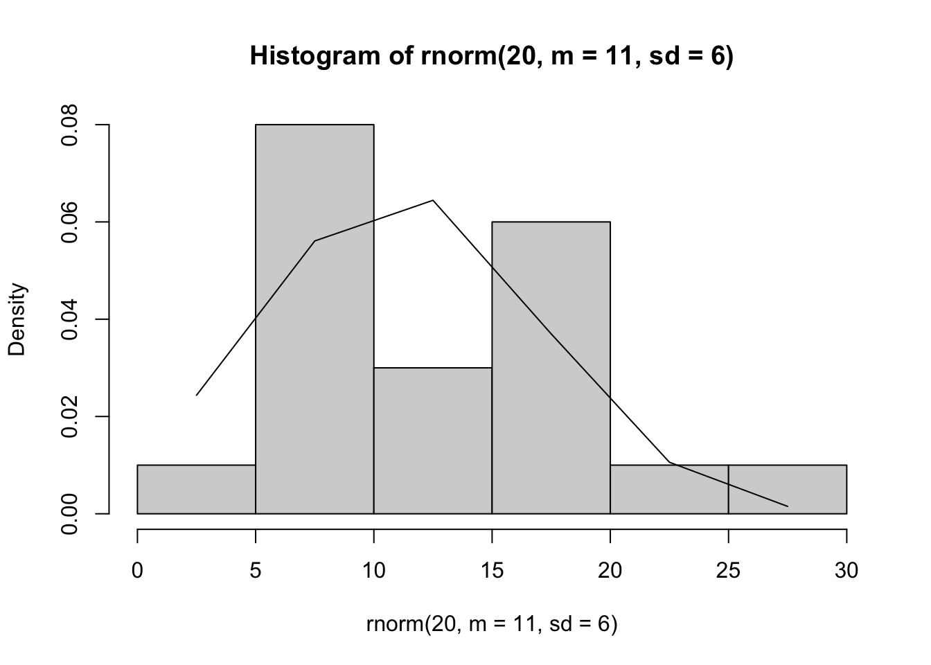

$*Histogram of random numbers drawn from a normal distribution with $\mu=11$ and $\sigma=6$. The normal probability density function is drawn as well.*$

Figure 14.1: Histogram of random numbers drawn from a normal distribution with $\mu=11$ and $\sigma=6$. The normal probability density function is drawn as well.

14.5 Numerical integration of ordinary differential equations

In order to study continuous population dynamics, we often would like to integrate complex nonlinear functions of population dynamics. To do this, we need to use numerical techniques that turn the infinitely small steps of calculus, $\d x$, into very small, but finite steps, in order to approximate the change in $y$, given the change in $x$, or $dy/dx$. Mathematicians and computer scientists have devised very clever ways of doing this very accurately and precisely. In R, the best package for this is deSolve, which contains several solvers for differential equations that perform numerical integration. We will access these solvers (i.e. numerical integraters) using the ode function in the deSolve package. This function, ode, is a “wrapper” for the underlying suite of functions that do the work. That is, it provides a simple way to use any one of the small suite of functions.

When we have an ordinary differential equation (ODE) such as logistic growth, $dN/dt = rN(1-\alpha N)$, we say that we “solve” the equation for a particular time interval given a set of parameters and initial conditions or initial population size. For instance, we say that we solve the logistic growth model for time at $t=0,\, 1 \ldots \, 20$, with parameters $r=1$, $\alpha=0.001$, and $N_0=10$.

Let’s do an example with ode, using logistic growth. We first have to define a function in a particular way. The arguments for the function must be time, a vector of populations, and a vector or list of model parameters.

logGrowth <- function(t, y, p){
  N <- y[1]
  with(as.list(p), {
    dN.dt <- r * N * (1 - a * N)
    return( list( dN.dt ) )
  } )
}

Note that I like to convert $y$ into a readable or transparent state variable ($N$ in this case). I also like to use with which allows me to use the names of my parameters (Petzoldt:2003dp?); this works only is p is a vector with named paramters (see below). Finally, we return the derivative as a list of one component.

The following is equivalent, but slightly less readable or transparent.

  logGrowth <- function(t, y, p){
    dN.dt <- p[1] * y[1] * (1 - p[2] * y[1])
    return( list( dN.dt ) )
  }

This requires that the order of the parameters is expected, that $r$ is first and $\alpha$ is second.

To solve the ODE, we will need to specify parameters, and initial conditions. Because we are using a vector of named parameters, we need to make sure we name them! We also need to supply the time steps we want.

p <- c(r=1, a = 0.001)
y0 <- c(N=10)
t <- 1:20

Now you put it all into ode, with the correct arguments. The output is a matrix, with the first column being the time steps, and the remaining being your state variables. First we load the deSolve package.

library(deSolve)
out <- ode(y=y0, times=t, func=logGrowth, parms=p)
out[1:5,]

##      time         N
## [1,]    1  10.00000
## [2,]    2  26.72369
## [3,]    3  69.45310
## [4,]    4 168.66426
## [5,]    5 355.46079

plot(out)

If you are going to model more than two species, y becomes a vector of length 2. Here we create a function for Lotka-Volterra competition, where \[\frac{d N_1}{d t} = r_1 N_1\left(1 - \alpha_{11} N_1 - \alpha_{12} N_2 \right)\] \[\frac{d N_2}{d t} = r_2N_2\left(1 - \alpha_{22}N_2 - \alpha_{21}N_1 \right)\]

LVComp <- function(t, y, p){
  N <- y
  with(as.list(p), {
    dN1.dt <- r[1] * N[1] * (1 - a[1,1]*N[1] - a[1,2]*N[2])
    dN2.dt <- r[2] * N[2] * (1 - a[2,1]*N[1] - a[2,2]*N[2])
    return( list( c(dN1.dt, dN2.dt) ) )
  } )
}

Note that LVComp assumes that $N$ and $r$ are vectors, and the competition coefficients are in a matrix. For instance, the function extracts the the first element of r for the first species (r[1]); for the intraspecific competition coefficient for species 1, it uses the element of a that is in the first column and first row (a[1,1]). The vector of population sizes, $N$, contains one value for each population at one time point. Thus here, the vector contains only two elements (one for each of the two species); it holds only these values, but will do so repeatedly, at each time point. Only the output will contain all of the population sizxes through time.

To integrate these populations, we need to specify new initial conditions, and new parameters for the two-species model.

a <- matrix(c(0.02, 0.01, 0.01, 0.03), nrow=2)
r <- c(1,1)
p2 <- list(r, a)
N0 <- c(10,10)
t2 <- c(1,5,10,20)
out <- ode(y=N0, times=t2, func=LVComp, parms=p2)
out[1:4,]

##      time        1        2
## [1,]    1 10.00000 10.00000
## [2,]    5 35.53914 21.79929
## [3,]   10 39.61141 20.35672
## [4,]   20 39.99332 20.00667

plot(out)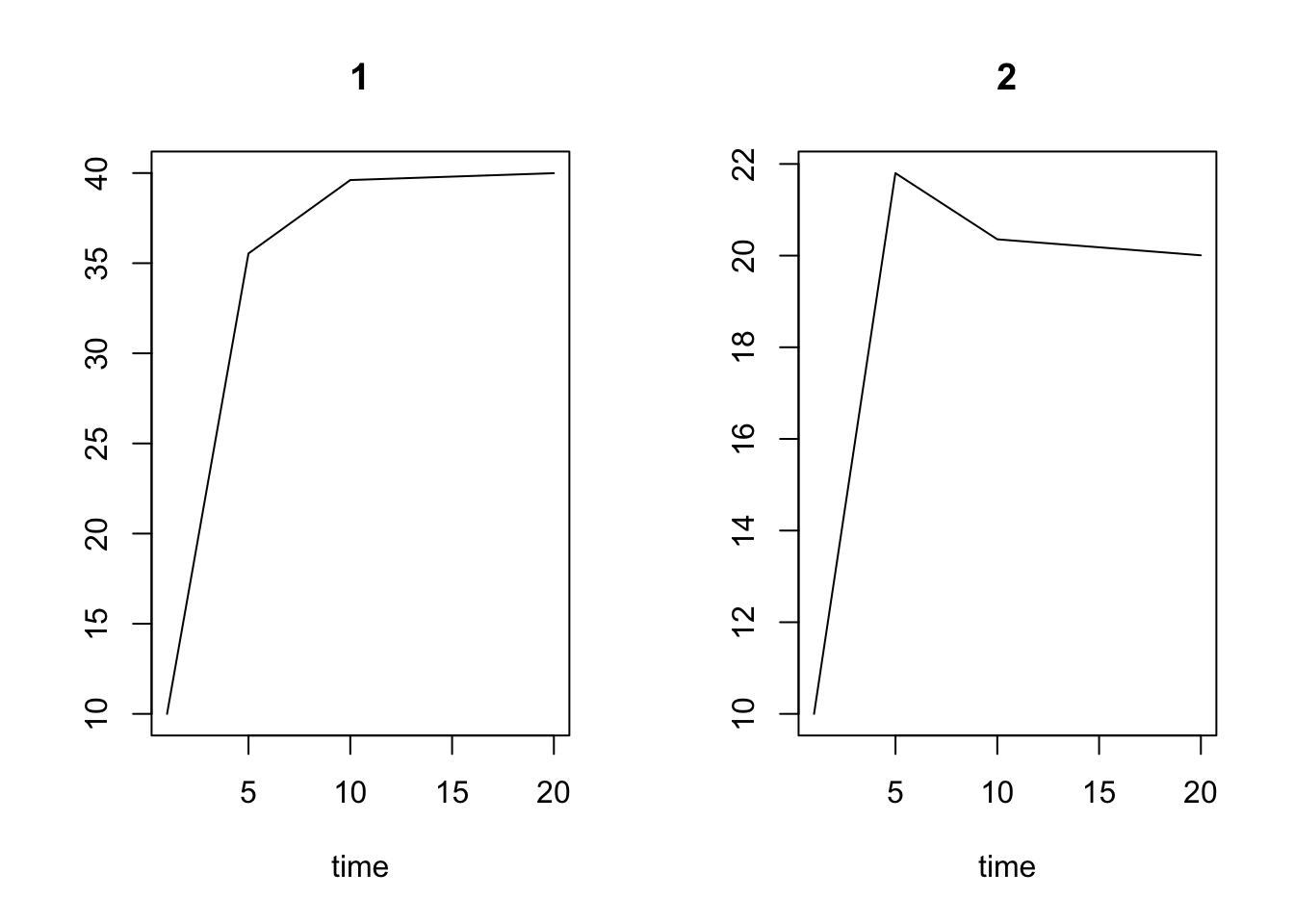

The ode function is a wrapper for a variety of ODE solvers; the default lsoda is a well tested tool. In addition, it has several bells and whistles that we will not need to take advantage of here, although I will mention one,hmax. This tells lsoda the largest step it can take. Once in a great while, with a very stiff ODE (a very wiggly complex dynamic), ODE assumes it can take a bigger step than it should. Setting hmax to a smallish number will limit the size of the step to help ensure that the integration proceeds as it should.

One of the other solvers in the deSolve, lsodar, will also return roots (or equilibria), for a system of ODEs, if they exist. Here we find the roots (i.e. the solutions, or equilibria) for a two species enemy-victim model.

EV <- function(t, y, p){
  with(as.list(p), {
    dv.dt <- b * y[1]*(1-.005*y[1]) - a*y[1]*y[2]
    de.dt <-a*e*y[1]*y[2] - s*y[2]
    return( list( c(dv.dt, de.dt) ) )
  } )
}

To use lsodar to find equilibria, we need to specify a root finding function whose inputs are are the sme of the ODE function, and which returns a scalar (a single number) that determines whether the rate of change ($dy/dx$) is sufficiently close to zero that we can say that the system has stopped changed, that is, has reached a steady state or equilibrium. Here we sum the absolute rates of change of each species, and then subtract 10$^{-10}$; if that difference is zero, we decide that, for all pratcial purposes, the system has stopped changing.

rootfun <- function (t,y,p) { 
dstate <- unlist(EV(t,y,p)) #rate of change vector 
return(sum(abs(dstate))-1e-10) 
}

Note that unlist changes the list returned by EV into a simple vector, which can then be summed.

Next we specify parameters, and time. Here all we want is the root, so we specify that we want the value of $y$ after a really long time ($t=10^{10}$). The lsodar function will stop sooner than that, and return the equilibrium it finds, and the time step at which it occurred.

p <- c(b = 0.5, a = 0.02, e=0.1, s=0.2)
t <- c(0,1e10)

Now we run the function.

out <- ode(y=c(45,200), t, EV, parms=p, rootfun=rootfun, method="lsodar")
out[,]

##          time   1     2
## [1,]   0.0000  45 200.0
## [2,] 500.8094 100  12.5

Here we see that the steady state population sizes are $V=100$ and $E=12.5$, and that given our starting point, this steady state was achieved at $t=500.8$. Other information is available; see ?lsodar after loading the deSolve package.

We can also find the equilibrium or steady state using the rootSolve package.

library(rootSolve)
equil <- runsteady(y=c(45,200), times=c(0,1E5), func=EV, parms=p)
round(equil$y, 3)

## [1] 100.0  12.5

14.6 Eigenanalysis

Performing eigenanalysis in R is easy. We use the function which returns a list with two components. The first named component is a vector of eigenvalues and the second named component is a matrix of corresponding eigenvectors. These will be numeric if possible, or complex, if any of the elements are complex numbers.

Here we have a typical demographic stage matrix.

A <- matrix(c(0, .1, 10, .5), nrow=2)
eig.A <- eigen(A)
str(eig.A)

## List of 2
##  $ values : num [1:2] 1.281 -0.781
##  $ vectors: num [1:2, 1:2] -0.9919 -0.127 -0.997 0.0778
##  - attr(*, "class")= chr "eigen"

Singular value decomposition (SVD) is a generalization of eigenanalysis and is used in R for some applications where eigenanalysis was used historically, but where SVD is more numerically accurate ( for principle components analysis).

14.6.1 Eigenanalysis of demographic versus Jacobian matrices

Eigenanalyses of demographic and Jacobian matrices are worth comparing. In one sense, they have similar meanings — they both describe the asymptotic (long-term) properties of a system, either population size (demographic matrix) or a perturbation at an equilibrium. The quantitative interpretation of the eigenvalues will therefore differ.

In the case of the stage (or age) structured demographic model, the elements of the demographic matrix are discrete per capita increments of change over a specified time interval. This is directly analogous to the finite rate of increase, $\lambda$, in discrete unstructured models. (Indeed, an unstructured discrete growth model is a stage-structured model with one stage). Therefore, the eigenvalues of a demographic matrix will have the same units — a per capita increment of change. That is why the dominant eigenvalue has to be greater than 1.0 for the population to increase, and less than 1 (not merely less than zero) for the population to decline.

In the case of the Jacobian matrix, comprised of continuous partial differential equations, the elements are per capita instantaneous rates of change. As differential equations, they describe the instantanteous rates of change, analogous to $r$. Therefore, values greater than zero indicate increases, and values less than zero indicate decreases. Because these rates are evaluated at an equilibrium, the equilibrium acts like a new zero — positive values indicate growth away from the equilibrium, and negative values indicate shrinkage back toward the equilibrium. When we evaluate these elements at the equilibrium, the numbers we get are in the same units as $r$, where values greater than zero indicate increase, and values less than zero indicate decrease. The change they describe is the instantaneous per capita rate of change of each population with respect to the others. The eigenvalues summarizing all of the elements Jacobian matrix thus must be less than zero for the disturbance to decline.

So, in summary, the elements of a demographic matrix are discrete increments over a real time interval. Therefore its eigenvalues represent relative per capita growth rates a discrete time interval, and we interpret the eigenvalues with respect to 1.0. On the other hand, the elements of the Jacobian matrix are instantaneous per captia rates of change evaluated at an equilibrium. Therefore its eigenvalues represent the per capita instantaneous rates of change of a tiny perturbation at the equilibrium. We interpret the eigenvalues with respect to 0 indicating whether the perturbation grows or shrinks.

14.7 Derivation of the right eigenvalues

\[\begin{align*} Aw &=\lambda w\\ Aw-\lambda w &=0\\ Aw - \lambda I w &=\mathbf{0} \\ \left(A - \lambda I\right)w &=0 \end{align*}\]

By rules of determinants, it follows then that, \[\mathrm{det} \left| A - \lambda I \right| =0\]

And here is an empirical example.

A <- matrix(1:4, nrow=2)
lambda <- eigen(A)$values[1]
w <- eigen(A)$vectors[,1]
I <- diag(c(1,1))
round(lambda*w - A%*%w, 4)

##      [,1]
## [1,]    0
## [2,]    0

round(lambda*I%*%w - A%*%w, 4)

##      [,1]
## [1,]    0
## [2,]    0

round((lambda*I - A)%*%w, 4)

##      [,1]
## [1,]    0
## [2,]    0

det( lambda*I-A )

## [1] 0

Once we know that the determinant is zero, we can use that to create a simple quadratic equation in terms of $\lambda$, and then solve. First, let’s remember what the above difference is: \[\mathbf{A} - \lambda\mathbf{I} = \begin{pmatrix} a-\lambda & b \\ c & d - \lambda \end{pmatrix}\]

Then we can use the determinant to solve for lambda. \[ \mathrm{det} \begin{pmatrix} a-\lambda & b \\ c & d - \lambda \end{pmatrix} = (a-\lambda)(d-\lambda) - bc = 0\] \[\lambda^2 - (a+d)\lambda + (ad-bc) = 0\] \[\lambda = \frac{-(a+d) \pm \sqrt{(a+d)^2 - 4(ad-bc)}}{2}\] And that is one way to find the two eigenvalues of a $2 \times 2$ matrix, whether it is a demographic projection matrix, predator-prey interaction matrix, or something else.

14.8 Symbols used in this book

I am convinced that one of the biggest hurdles to learning theoretical ecology — and the one that is easiest to overcome — is to be able to “read” and hear them in your head. This requires being able to pronounce Greek symbols. Few of us learned how to pronounce $\alpha$ in primary school. Therefore, I provide here an incomplete simplistic American English pronunciation guide for (some of) the rest of us, for symbols in this book. Only a few are tricky, and different people will pronounce them differently.

Symbols and their pronunciation; occasional usage applies to lowercase, unless otherwise specified. A few symbols have common variants. Any symbol might be part of any equation; ecologists frequently ascribe other meanings which have to be defined each time they are used.

Table 14.1: Symbols and their pronunciation; occasional usage applies to lowercase, unless otherwise specified. A few symbols have common variants. Any symbol might be part of any equation; ecologists frequently ascribe other meanings which have to be defined each time they are used.
Greek Symbol	Spelling and pronunciation
A, $\alpha$	alpha; al’-fa; point or local diversity (or a parameter in the logseries abundance distribution)
B, $\beta$	beta; bay’-ta; turnover diversity
$\mathrm{\Gamma}$, $\gamma$	gamma; gam’-ma; regional diversity
$\mathrm{\Delta}$, $\delta$, $\partial$	delta; del’-ta; change or difference
E, $\epsilon$, $\varepsilon$	epsilon; ep’-si-lon; error
$\mathrm{\Theta}$, $\theta$	theta; thay’-ta (‘th’ as in ‘thanks’); in neutral theory, biodiversity
$\mathrm{\Lambda}$, $\lambda$	lambda; lam’-da; eigenvalues, and finite rate of increase
M, $\mu$	mu; meeoo, myou; mean
N, $\nu$	nu; noo, nou
$\mathrm{\Pi}$, $\pi$	pi; pie; uppercase for product (of the elements of a vector)
P, $\rho$	rho; row (as in ‘a boat’); correlation
$\mathrm{\Sigma}$, $\sigma$, $\varsigma$	sigma; sig’-ma; standard deviation (uppercase is used for summation)
T, $\tau$	tau; (sounds like what you say when you stub your toe - ‘Ow!’ but with a ‘t’).
$\Phi$, $\phi$	phi; fie, figh
X, $\chi$	chi; kie, kigh
$\mathrm{\Psi}$, $\psi$	psi; sie, sigh
$\mathrm{\Omega}$, $\omega$	omega; oh-may’-ga; degree of omnivory

13 Diversity

15 References

Greek Symbol	Spelling and pronunciation
A, \(\alpha\)	alpha; al’-fa; point or local diversity (or a parameter in the logseries abundance distribution)
B, \(\beta\)	beta; bay’-ta; turnover diversity
\(\mathrm{\Gamma}\), \(\gamma\)	gamma; gam’-ma; regional diversity
\(\mathrm{\Delta}\), \(\delta\), \(\partial\)	delta; del’-ta; change or difference
E, \(\epsilon\), \(\varepsilon\)	epsilon; ep’-si-lon; error
\(\mathrm{\Theta}\), \(\theta\)	theta; thay’-ta (‘th’ as in ‘thanks’); in neutral theory, biodiversity
\(\mathrm{\Lambda}\), \(\lambda\)	lambda; lam’-da; eigenvalues, and finite rate of increase
M, \(\mu\)	mu; meeoo, myou; mean
N, \(\nu\)	nu; noo, nou
\(\mathrm{\Pi}\), \(\pi\)	pi; pie; uppercase for product (of the elements of a vector)
P, \(\rho\)	rho; row (as in ‘a boat’); correlation
\(\mathrm{\Sigma}\), \(\sigma\), \(\varsigma\)	sigma; sig’-ma; standard deviation (uppercase is used for summation)
T, \(\tau\)	tau; (sounds like what you say when you stub your toe - ‘Ow!’ but with a ‘t’).
\(\Phi\), \(\phi\)	phi; fie, figh
X, \(\chi\)	chi; kie, kigh
\(\mathrm{\Psi}\), \(\psi\)	psi; sie, sigh
\(\mathrm{\Omega}\), \(\omega\)	omega; oh-may’-ga; degree of omnivory