5 Describing a nitrogen budget
5.1 Learning Objectives
By the end of this chapter, you should be able to:
- Translate a published nitrogen budget into a compartment model diagram
- Write balance equations for multi-compartment systems with mixed rate types
- Distinguish between first-order and zero-order fluxes in a real ecosystem
- Estimate model parameters from literature data using both incremental and instantaneous rate methods
- Understand why we use instantaneous rates in differential equations
- Implement and run a multi-compartment model in R
- Interpret model output in terms of ecosystem dynamics and equilibrium states
- Add self-limitation to represent biological constraints on growth
5.2 Background Readings
- pp. 17-35 (Soetaert and Hermann 2009)
- Bormann et al. 1977. Nitrogen Budget for an aggrading northern hardwood forest ecosystem. Science 196:981-983.
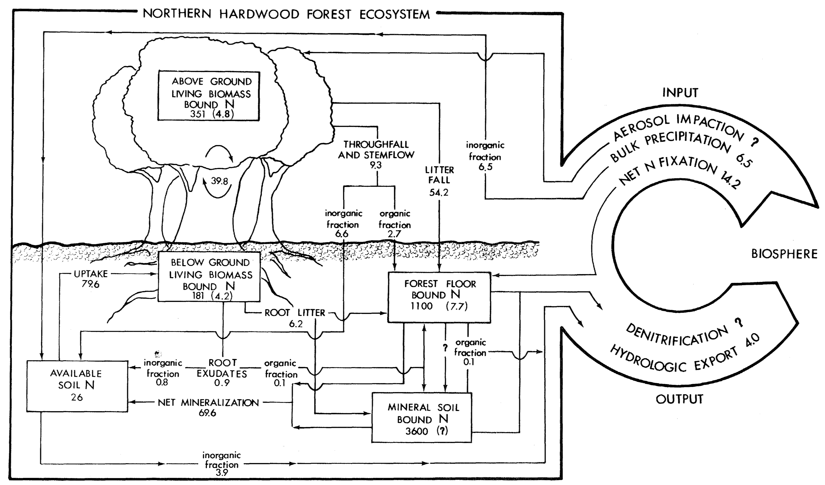
Figure 5.1: Nitrogen budget for a temperate northern hardwood forest (Hubbard Brook Watershed 6, Bormann et al. 1977).
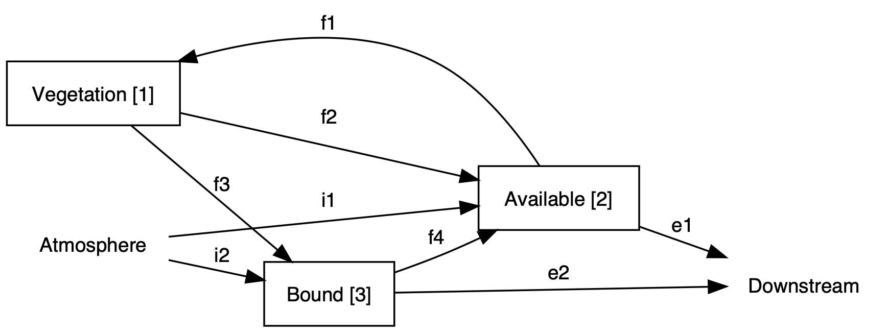
Figure 5.2: A simpler compartment model for Hubbard Brook Watershed 6, based on Bormann et al. (1977).
5.3 Understanding the Hubbard Brook System
Before we dive into the mathematics, let’s think about what’s actually happening in this forest ecosystem. Hubbard Brook is a classic study site where ecologists have tracked nutrient cycling in a northern hardwood forest for decades. This particular watershed (Watershed 6) was recovering from logging - an aggrading forest actively accumulating biomass and nutrients.
The vegetation compartment (V) represents all living plant tissue - leaves, wood, fine roots. Plants are actively taking up nitrogen from the soil to build proteins and other molecules. As this forest regrows, the vegetation pool is increasing.
The available pool (A) is nitrogen in forms plants can use immediately - primarily ammonium (NH₄⁺) and nitrate (NO₃⁻) dissolved in soil water. This pool is relatively small but turns over quickly. Think of it as the “checking account” that plants draw from.
The bound pool (B) is organic nitrogen locked up in dead organic matter - fallen leaves, dead roots, humus. This is the largest pool but changes slowly - like a “savings account” that releases nutrients gradually through decomposition. Most of the forest’s nitrogen is stored here.
Key insight: Not all fluxes operate the same way. Some depend on how much material is available (first-order kinetics), while others are more constant (zero-order kinetics). Recall from Chapters 2 and 3 that we learned about both types. This real ecosystem combines both. As we build our model, think about which biological processes fit each pattern.
5.4 Getting started
- (S&H 15-17) For any ecosystem, we want to start with paper and pencil and sketch out the pools and the fluxes that we think are important (see example, Fig. 5.2). Don’t sweat the details yet – you’ll revise it anyway. Go ahead and label the compartments and the fluxes with both biological and physical processes as well as some simple abstract notation.
5.5 Classifying the Fluxes
Before writing balance equations, let’s classify each flux by its kinetics. This connects directly to what you learned in the previous chapters.
Zero-order (constant) fluxes:
- Bulk precipitation (I₁): Rain and snow deposit nitrogen regardless of how much N is already in the forest. This is an external input to the system.
- N fixation (I₂): Symbiotic bacteria in root nodules convert atmospheric N₂ to usable forms. The rate depends on bacterial activity and environmental conditions, not on existing forest N pools.
First-order (mass-dependent) fluxes:
- Plant uptake (f₁): Depends on both available N (more available = faster uptake) and plant biomass (more roots = more uptake capacity). This is a second-order interaction: f₁ = function(A,V).
- Throughfall/exudates (f₂): Rain washes N out of leaves and roots release organic compounds. Proportional to vegetation biomass: more vegetation = more throughfall.
- Litterfall (f₃): Leaf and root senescence. Proportional to vegetation biomass - larger forests produce more litter.
- Mineralization (f₄): Decomposers break down organic matter, releasing available N. Rate depends on how much organic matter is present - more substrate = faster mineralization.
- Stream export from A (E₁): Dissolved N washes out with streamflow. Proportional to concentration, which depends on pool size.
- Stream export from B (E₂): Particulate organic matter washed downstream. Proportional to the bound pool.
Why does this matter? The mathematical form of each term in our equations will match its kinetic type. Recognizing this pattern helps you write the equations correctly and understand why they have the forms they do. Zero-order processes appear as constants in equations; first-order processes appear as rate constant × pool size.
5.5.1 Quick Check 1
Before moving on, make sure you understand:
- Which fluxes in Figure 5.2 are external to the three-compartment system (cross system boundaries)?
- Which fluxes are internal transfers (stay within the system)?
- For each internal flux, which compartment is the source and which is the sink?
Click for answers
External inputs: I₁ (precipitation to A), I₂ (fixation to B)
External outputs: E₁ (export from A), E₂ (export from B)
Internal transfers: - f₁: from A to V (plant uptake) - f₂: from V to A (throughfall/exudates) - f₃: from V to B (litterfall) - f₄: from B to A (mineralization)
5.6 Write Balance Equations
Recall from Chapter 4 that a balance equation is simply: Change in pool = Sources - Sinks
For each compartment, we identify all arrows entering (sources) and leaving (sinks), then write the rate equation. Here are the balance equations for Fig. 5.2:
Rate of change of vegetation = uptake - exudates and throughfall - leaf and root litter loss \[\frac{dV}{dt} = f_1 - f_2 - f_3\]
Rate of change in available pool = bulk precip + exudates and throughfall + net mineralization - uptake - stream export \[\frac{dA}{dt} = I_1 + f_2 + f_4 - f_1 - E_1\]
Rate of change in the bound pool = net N fixation + leaf and root litter loss - net mineralization - stream export \[\frac{dB}{dt} = I_2 + f_3 - f_4 - E_2\]
5.6.1 Quick Check 2
Before looking ahead:
For the vegetation equation, identify which terms represent:
- Gains to the pool
- Losses from the pool
- Transfers within the system vs. external inputs/outputs
Sum all three balance equations. What should cancel out? What should remain?
Does this match the total mass budget we’ll show next?
Click for answers
Gains: f₁ (internal transfer from A); Losses: f₂ and f₃ (internal transfers to A and B); External: none for vegetation - it only exchanges with other compartments, not with outside the system
When you sum the three equations, all internal fluxes (f₁, f₂, f₃, f₄) should appear once positive and once negative, so they cancel. Only external inputs and outputs remain.
Yes! See the next section.
5.7 Assess the Total System Budget
For Fig. 5.2, we have the total rate of change for the entire system:
\[\frac{d\left(V+A+B\right)}{dt} = \frac{dV}{dt} + \frac{dA}{dt} + \frac{dB}{dt}\]
Substituting our balance equations:
\[\frac{d\left(V+A+B\right)}{dt} = (f_1 - f_2 - f_3) + (I_1 + f_2 + f_4 - f_1 - E_1) + (I_2 + f_3 - f_4 - E_2)\]
Now watch what happens when we rearrange and cancel terms:
\[\frac{d\left(V+A+B\right)}{dt} = I_1 + I_2 + f_1 - f_1 + f_2 - f_2 + f_3 - f_3 + f_4 - f_4 - E_1 - E_2\]
All the internal fluxes cancel (this is the key feature of mass balance!):
\[\frac{d\left(V+A+B\right)}{dt} = I_1 + I_2 - E_1 - E_2\]
From this we see that the total mass budget for this watershed depends simply on imports (inputs) and exports (outputs). The internal cycling doesn’t affect the total - it just redistributes nitrogen among compartments. This is a powerful check on our model - if the internal fluxes don’t cancel when we sum everything, we made a mistake!
5.8 Mathematical Forms for Fluxes
Now we need to express each flux as a mathematical function. Recall from earlier that we classified fluxes as zero-order or first-order. Now we make that explicit.
For zero-order (constant) fluxes:
These are simply constants. From the data: - I₁ = 6.5 kg N ha⁻¹ y⁻¹ (precipitation) - I₂ = 14.2 kg N ha⁻¹ y⁻¹ (fixation)
For first-order fluxes:
A common starting point for dynamics depending on pool sizes is the law of mass action. This states that the reaction rate is proportional to the amount of substrate present in a single pool.
For a flux depending on one pool: flux = k × Pool
For second-order fluxes:
A flux is second-order when a rate is proportional to either two pools (\(XY\)), or to the the square of one pool (\(X^2\)). This still relies ofn the law of law of mass action.
For a flux depending on two pools: flux = k × Pool₁ × Pool₂
Using mass action kinetics, we express the fluxes in our N budget (Fig. 5.2) as:
- f₁ (uptake): depends on both A and V → f₁ = a₁ × A × V
- f₂ (throughfall/exudates): depends on V → f₂ = a₂ × V
- f₃ (litterfall): depends on V → f₃ = a₃ × V
- f₄ (mineralization): depends on B → f₄ = a₄ × B
- E₁ (export from A): depends on A → E₁ = a₅ × A
- E₂ (export from B): depends on B → E₂ = a₆ × B
5.8.1 Complete Balance Equations
Substituting these mathematical forms into our balance equations:
\[\begin{align} \frac{dV}{dt} &= a_{1}AV - a_{2}V - a_3 V\\ \frac{dA}{dt} &= I_1 + a_{2}V + a_{4}B - a_{1}AV - a_{5}A\\ \frac{dB}{dt} &= I_2 + a_{3}V - a_{4}B - a_{6}B \end{align}\]
Take time to identify each term and think about the biology or physics that might govern it. For instance, why does uptake depend on both A and V? Because you need both nutrients available AND plant tissue capable of taking them up.
5.9 A Critical Detail: Consistent Sign Conventions
Before we estimate parameters, we need to address an important mathematical detail that can cause confusion.
The challenge: When we estimate parameters from loss fluxes using real data, we often get negative numbers (because the pool is declining). But when we write equations, we need to be careful about signs.
Two approaches:
Option 1 - Keep the signs in the parameters:
a₄ = -0.0149  # negative because it's a loss from B
dB/dt = ... + a₄*B  # add the negative rate
Option 2 - Use absolute values (we’ll use this):
a₄ = 0.0149  # store as positive magnitude
dB/dt = ... - a₄*B  # subtract explicitly in equation
Why Option 2? It makes the biology clearer in our equations. When we see “- a₄ × B” in the equation for dB/dt, we immediately know this is a loss from B. The signs in our equations match our conceptual diagram - sources have + signs, sinks have - signs.
Our rule: We’ll calculate the magnitude (absolute value) of all rate constants and use +/- signs in equations to show direction of transfer. This matches the visual logic of our box-and-arrow diagrams.
5.10 Parameterization
Parameterization is what we call assigning numerical values to mathematical parameters. Here, we find initial estimates for the parameters in our model. We use the literature for this purpose (Bormann, Likens, and Melillo 1977).
The data from Bormann et al. give us annual fluxes (kg N ha⁻¹ y⁻¹) and pool sizes (kg N ha⁻¹). Our job is to convert these observations into rate constants.
5.10.1 The Challenge: Annual Rates vs. Instantaneous Rates
The problem we face: Our data from Bormann give us annual budgets - total amounts that moved over one year. But differential equations describe instantaneous rates - how fast things are changing at any given moment in time.
An analogy to clarify this:
Imagine you’re driving. Your odometer shows you drove 60 miles in one hour - that’s like an annual rate, total distance over total time. But you didn’t drive exactly 60 mph the entire time - you accelerated from stoplights, slowed in traffic, cruised on the highway. Your speedometer shows your instantaneous speed at each moment - that’s what we need for differential equations.
In our model:
If the bound pool loses 69.6 kg N ha⁻¹ year⁻¹ to mineralization, we can’t just write:
\[\frac{dB}{dt} = \ldots - 69.6\]
Why not? Two reasons:
Units don’t match: The left side has units of kg ha⁻¹ y⁻¹, but we said the flux depends on pool size: f₄ = a₄ × B. If B has units of kg ha⁻¹, then a₄ must have units of y⁻¹ (per year), not kg ha⁻¹ y⁻¹.
The rate changes: As the pool shrinks or grows during the year, the actual rate of loss changes if the flux is proportional to pool size. We need the instantaneous proportionality constant, not the average annual flux.
Two approaches to estimate rate constants:
5.10.2 Approach 1: Annual Incremental Rates (Simpler)
For a simple approximation, we can calculate an annual incremental rate by dividing the annual flux by the pool size:
\[\text{rate constant} = \frac{\text{annual flux}}{\text{current pool size}}\]
Example: Net mineralization from the bound pool
The bound pool (B) loses 69.6 kg N ha⁻¹ y⁻¹ to mineralization, and currently contains 4,700 kg N ha⁻¹.
\[\begin{align*} F_4 &= a_4 B\\ 69.6 &= a_4 \times 4700\\ a_4 &= \frac{69.6}{4700}\\ a_4 &\approx 0.0148 \text{ y}^{-1} \end{align*}\]
Example: Plant uptake (second-order reaction)
We use the same approach for second-order equations. The vegetation gains 79.6 kg N ha⁻¹ y⁻¹ through uptake. The available pool contains 26 kg N ha⁻¹ and vegetation contains 532 kg N ha⁻¹.
\[\begin{align*} F_1 &= a_1 AV \\ 79.6 &= a_1 \times 26 \times 532 \\ a_1 &= \frac{79.6}{26 \times 532}\\ a_1 &\approx 0.0058 \text{ (kg ha}^{-1})^{-1} \text{y}^{-1} \end{align*}\]
Note the units! For a second-order rate constant, we have (kg ha⁻¹)⁻¹ y⁻¹, which makes the units work out when we multiply by two pools.
5.10.3 Approach 2: Instantaneous Rates Using Logarithms (More Accurate)
For a more accurate approach that properly handles the continuous nature of differential equations, we use logarithms. This approach gives us true instantaneous rate constants.
The mathematical basis:
If a pool changes continuously at a rate proportional to its size, then:
\[\text{instantaneous rate constant} = \ln\left(\frac{\text{pool after change}}{\text{pool before change}}\right)\]
For our system, if we imagine the pool over one year with only one flux operating:
Example: Net mineralization (loss from bound pool)
Let B₀ be the mass of N in the bound pool at time 0, and B₁ would be the mass one year later if we account for only the mineralization flux coming out of B:
\[B_0=4700 \quad ; \quad B_1 = B_0 - F_4 = 4700 - 69.6 = 4630.4\]
The instantaneous rate constant α₄ required to get us from B₀ to B₁ in one year is:
\[\alpha_4 = \ln\left(\frac{B_1}{B_0}\right) = \ln\left(\frac{4700-69.6}{4700}\right) \approx -0.0149 \text{ y}^{-1}\]
Notice: This gives us a negative number because the pool is declining. Following our sign convention from earlier, we’ll take the absolute value and use subtraction in the equation.
Comparing the two approaches:
- Annual incremental: a₄ = 0.0148 y⁻¹
- Instantaneous: |α₄| = 0.0149 y⁻¹
They’re very similar! For small changes relative to pool size, the two approaches give nearly identical results. However, for larger fractional changes, the instantaneous rate is more accurate for use in differential equations.
Why use logarithms? This comes from calculus. When a quantity changes exponentially (like radioactive decay or first-order chemical reactions), the instantaneous rate constant is exactly ln(final/initial) per unit time. Since our differential equations assume continuous exponential-like change, this is the theoretically correct approach.
5.10.4 Quick Check 3
Before looking at the full parameter table, try this yourself:
Calculate the parameter for throughfall and exudates (a₂) using both approaches:
- Annual flux from V to A: 6.6 + 0.8 = 7.4 kg N ha⁻¹ y⁻¹
- Current vegetation: 532 kg N ha⁻¹
- Show your work for both the incremental and instantaneous approaches
- Don’t forget the sign convention!
Click for answers
Incremental approach: \[a_2 = \frac{7.4}{532} = 0.0139 \text{ y}^{-1}\]
Instantaneous approach: \[\alpha_2 = \left|\ln\left(\frac{532 - 7.4}{532}\right)\right| = \left|\ln(0.9861)\right| = |-0.0140| = 0.0140 \text{ y}^{-1}\]
Again, very similar values!
5.11 Calculating All Parameters in R
Now let’s calculate all our parameters systematically. Following our sign convention, we’ll compute absolute values and use the instantaneous rate approach (logarithmic method).
Throughfall and inorganic exudates - a loss from vegetation, so we use absolute value:
## [1] 0.01400742Litter, throughfall, organic exudates - a loss from vegetation to bound pool:
# Annual flux from V to B: 54.2 + 2.7 + 0.1 + 6.2 = 63.2 kg N/ha/y
a3 <- abs( log( (532 - 54.2 - 2.7 - 0.1 - 6.2) / 532) )
a3
## [1] 0.1264673Net mineralization - a loss from the bound pool:
## [1] 0.01491925Export from the available pool - a loss:
## [1] 0.1625189Export from the bound pool - a loss:
## [1] 2.127682e-05N Uptake by plants - a gain to vegetation that depends on both the source ($\() and sink (\)V\(), making it a second order rate. This makes the rate more difficult to approximate, because the flux simply moves from one pool (\)A\() to the other (\)V\() and does not leave completely. Therefore, we will fall back on the incremental approach. In this case, the rate depends on the *product* of the the two pools (\)AV$).
## [1] 0.005754772Now we create a single vector of all parameters, including the constant inputs:
params <- c(
  i1 = 6.5,   # bulk precipitation (kg N/ha/y)
  i2 = 14.2,  # N fixation (kg N/ha/y)
  a1 = a1,    # uptake rate constant
  a2 = a2,    # throughfall/exudates rate constant
  a3 = a3,    # litterfall rate constant
  a4 = a4,    # mineralization rate constant
  a5 = a5,    # export from available pool
  a6 = a6     # export from bound pool
)

# Display with nice formatting
round(params, 5)
## i1 i2 a1 a2 a3 a4 a5 a6
## 6.50000 14.20000 0.00575 0.01401 0.12647 0.01492 0.16252 0.000025.11.1 Parameter Table with Biological Interpretation
| Parameter | Biological Meaning | Units | Estimate |
|---|---|---|---|
| State Variables | |||
| V | Living vegetation (leaves, wood, roots) | kg N ha⁻¹ | 532 |
| A | Available N (NH₄⁺, NO₃⁻ in soil solution) | kg N ha⁻¹ | 26 |
| B | Bound N (organic matter, humus) | kg N ha⁻¹ | 4700 |
| Inputs (zero-order) | |||
| I₁ | Bulk precipitation input to A | kg N ha⁻¹ y⁻¹ | 6.5 |
| I₂ | Biological N fixation input to B | kg N ha⁻¹ y⁻¹ | 14.2 |
| Rate Constants (first-order) | |||
| a₁ | Plant uptake: A → V (depends on both pools) | (kg N ha⁻¹)⁻¹ y⁻¹ | 0.0057 |
| a₂ | Throughfall and exudates: V → A | y⁻¹ | 0.0140 |
| a₃ | Litterfall: V → B | y⁻¹ | 0.0126 |
| a₄ | Net mineralization: B → A | y⁻¹ | 0.0149 |
| a₅ | Stream export from A | y⁻¹ | 0.1620 |
| a₆ | Stream export from B | y⁻¹ | 0.000021 |
Note on measurement uncertainty: These parameters are derived from field measurements that have their own uncertainties. In a sensitivity analysis (Chapter ??), we would explore how uncertainty in these estimates affects model predictions. For now, we treat them as our best estimates.
5.12 Mathematical Solution
The mathematical solution is the process of making predictions using our model and our parameters. We solve the model. With simple models, we can sometimes find analytical solutions (like we did for steady states in Chapter 3). For most ecosystem models, we have to solve the models numerically using numerical integration - this is what computers excel at.
Here we write an R function that contains our system of differential equations. This will allow R’s ode() function from the deSolve package to integrate change through time.
library(deSolve)
library(tidyverse)

bormann1 <- function(t, y, p) {
  # Arguments:
  #   t = time (used by ode() even though not explicitly in our equations)
  #   y = vector of state variables (V, A, B)
  #   p = vector of parameters

  # We use as.list() to make both state variables and parameters
  # directly accessible by name
  with( as.list( c(y, p) ), {

    # The three balance equations
    # Notice: we use subtraction for losses (following our sign convention)
    dV.dt <- a1 * A * V - a2 * V - a3 * V
    dA.dt <- i1 + a2 * V + a4 * B - a1 * A * V - a5 * A
    dB.dt <- i2 + a3 * V - a4 * B - a6 * B

    # Return a LIST with two elements:
    # 1. Vector of rates (MUST be in same order as state variables)
    # 2. Additional outputs we want to track (total N in system)
    return(list(
      c(dV.dt, dA.dt, dB.dt),     # rates for V, A, B
      total = V + A + B            # total N for checking mass balance
    ))
  })
}
Understanding this function:
- The function takes three arguments that
ode()will provide - We use
with(as.list(...))so we can refer to variables by name (likeV,a1) instead of indexing (likey[1],p[3]) - Each equation matches our mathematical model, using - for losses and + for gains
- We return both the rates of change AND the total N (useful for verification)
Now we set up the simulation:
# Initial state: pool sizes from Bormann et al. (1977)
initial.state <- c(V = 532, A = 26, B = 4700)

# Time points: simulate for 20 years
time <- 0:20

# Solve the system
out <- ode(y = initial.state, times = time, func = bormann1, parms = params)

# Display first 6 time points
head(out)
## time V A B total
## [1,] 0 532.0000 26.00000 4700.000 5258.000
## [2,] 1 536.9206 25.96500 4711.487 5274.373
## [3,] 2 541.5310 25.82774 4723.405 5290.764
## [4,] 3 545.7697 25.70512 4735.701 5307.176
## [5,] 4 549.6810 25.59949 4748.326 5323.606
## [6,] 5 553.3077 25.50854 4761.236 5340.052What’s happening here:
ode()starts at year 0 with our initial state- At each time step, it calculates the rates using
bormann1() - It uses sophisticated numerical methods to integrate forward in time
- It returns a matrix with time in column 1, state variables in columns 2-4, and our custom output (total) in column 5
Let’s visualize these dynamics:
# Convert to long format for ggplot
outL <- out %>%
  as.data.frame() %>%
  pivot_longer(cols = -time, names_to = "State.var", values_to = "kg.N")

# Create the plot
ggplot(outL, aes(x = time, y = kg.N)) +
  geom_line(color = "blue", size = 1) +
  facet_wrap(~State.var, scales = "free_y") +
  labs(x = "Time (years)",
       y = "Nitrogen (kg N/ha)",
       title = "Hubbard Brook N Budget Dynamics") +
  theme_minimal()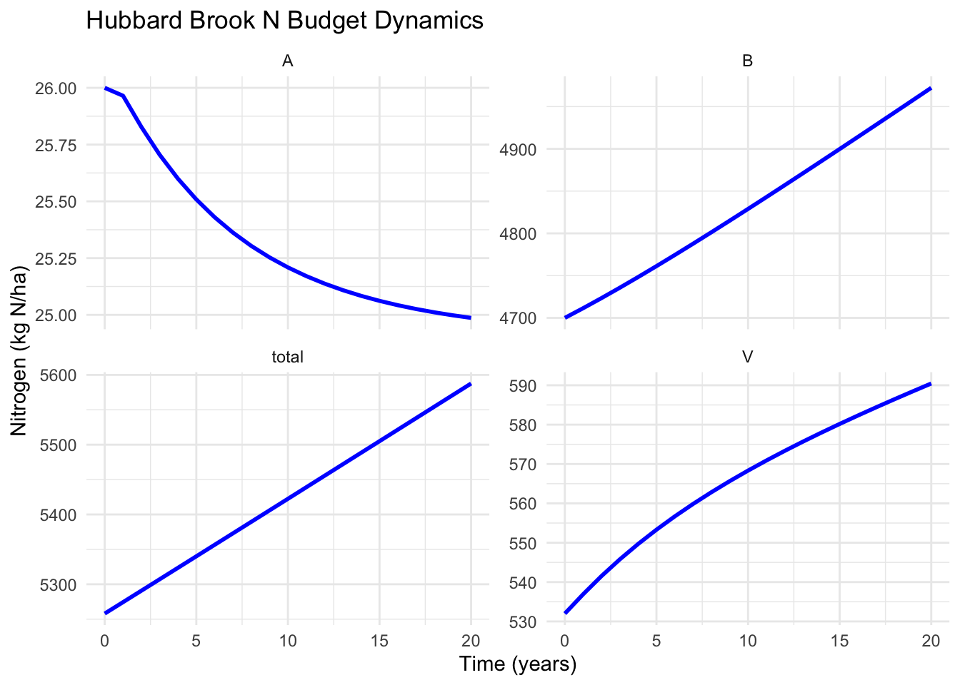
Figure 5.3: Dynamics of a simple N budget model based on Bormann et al. (1977). Each panel shows one compartment over 20 years.
5.13 Interpreting the Results
What do these trajectories tell us biologically?
1. Vegetation (V): Increases steadily over 20 years from 532 to about 680 kg N ha⁻¹.
Why? The uptake term (a₁ × A × V) exceeds the loss terms (a₂ × V + a₃ × V) when V is at these levels. The forest is actively regrowing - this is an aggrading system accumulating biomass after disturbance.
Notice: The rate of increase is slowing slightly - the curve is bending. This happens because as V grows, losses increase proportionally (more biomass → more litter), while uptake is limited by the declining available pool.
2. Available pool (A): Declines from 26 to about 18 kg N ha⁻¹.
Why? Vegetation is taking up more N than is being supplied by inputs (precipitation, mineralization). This makes ecological sense - an aggrading forest draws down the readily available nutrients. Plants are “mining” the available pool faster than it’s being replenished.
This creates a constraint: As A declines, the uptake rate (a₁ × A × V) will eventually slow even if V keeps growing.
3. Bound pool (B): Increases from 4,700 to about 4,950 kg N ha⁻¹.
Why? Litter inputs (a₃ × V) exceed mineralization losses (a₄ × B) as the forest grows. The forest is storing carbon and nutrients in organic matter. This is typical of forest development - dead organic matter accumulates.
4. Total system N: Increases from 5,258 to about 5,648 kg N ha⁻¹.
Why? Inputs (I₁ + I₂ = 20.7 kg N ha⁻¹ y⁻¹) exceed exports (which depend on pools and are currently small). The system is a net nitrogen sink.
5.13.1 The Key Problem
In this simple model, V would keep growing indefinitely. If you ran the simulation for 100 years, vegetation would continue accumulating nitrogen without bound.
That’s biologically unrealistic. Real forests reach maximum biomass limited by: - Light competition (trees shade each other) - Space constraints (finite area for roots and crowns) - Water and nutrient limitations - Disturbance (windthrow, pathogens, etc.)
This motivates our next refinement: adding self-limitation to represent biological carrying capacity.
5.13.2 Mass Balance Check
Let’s verify our model conserves mass correctly:
# Calculate total system inputs and outputs at initial conditions
inputs <- params["i1"] + params["i2"]
outputs_initial <- params["a5"] * initial.state["A"] + params["a6"] * initial.state["B"]

cat("Total inputs:", inputs, "kg N/ha/y\n")
## Total inputs: 20.7 kg N/ha/y## Initial outputs: 4.325493 kg N/ha/y## Net accumulation rate: 16.37451 kg N/ha/y# Check that total change matches inputs - outputs
# This is approximate because pools are changing
total_change <- out[nrow(out), "total"] - out[1, "total"]
time_elapsed <- max(time) - min(time)
avg_accumulation <- total_change / time_elapsed
cat("\nPredicted avg accumulation from model:", round(avg_accumulation, 2), "kg N/ha/y\n")##
## Predicted avg accumulation from model: 16.48 kg N/ha/yThe model’s accumulation rate is slightly less than inputs minus initial outputs because as pools change, export rates also change. This is correct behavior!
5.14 Exercise: Add Self-Limitation
The biological reality: As forests mature, growth slows even if nutrients remain available. Trees compete for light, space becomes limiting, and the ecosystem approaches a maximum biomass it can support - a carrying capacity.
This is a common pattern in ecology: populations and biomass pools show density-dependent growth - growth rate declines as density increases.
5.14.1 Your Task
Work through these steps before looking at the solution:
1. Conceptual step:
Where in the model should self-limitation appear? Think about which processes would slow down as vegetation approaches carrying capacity.
- Does precipitation become self-limiting? (No - rain falls regardless of forest biomass)
- Does litterfall become self-limiting? (No - more vegetation → more litter)
- Does plant growth become self-limiting? (Yes! This is the process to modify)
Write out the modified balance equation for dV/dt in words before you write the math.
2. Mathematical step:
The standard form for self-limitation is:
\[\text{growth rate} \times \left(1 - \frac{V}{K}\right)\]
where K is carrying capacity. Think about what this multiplier does: - When V = 0: multiplier = (1 - 0/K) = 1 (no limitation, full growth) - When V = K/2: multiplier = (1 - 0.5) = 0.5 (half of maximum growth) - When V = K: multiplier = (1 - K/K) = 0 (no growth, at carrying capacity)
In our current model, the net growth rate of vegetation is:
\[\frac{dV}{dt} = a_1 A V - a_2 V - a_3 V = (a_1 A - a_2 - a_3)V\]
Where should the self-limitation term go? Should it affect: - Just uptake (a₁ × A × V)? - Just net growth (the whole expression)? - Individual loss terms?
Hint: Biologically, self-limitation affects the net growth rate, not individual processes. Trees don’t stop dropping litter when crowded - they stop growing new tissue.
3. Parameterization:
We don’t have direct measurements of K from the Bormann data. We need to make an educated guess:
- The forest in 1977 had V = 532 kg N ha⁻¹
- This was a young, aggrading forest
- Mature northern hardwood forests might have 2-3× more biomass
Based on this reasoning, what’s a reasonable estimate for K? Try K = 600 as a starting point (only slightly higher than current), but think about what would happen with K = 800 or K = 1000.
4. Implementation:
Modify the bormann1 function to create bormann2. The change is small - just one multiplication in the dV.dt equation.
5. Simulation and interpretation:
- Run the model for 200 years (longer than before to see if it reaches equilibrium)
- Plot all three compartments
- Answer these questions:
- Do all three pools approach equilibrium?
- What are the equilibrium values?
- How long does it take to get close to equilibrium?
- What happens to the available pool as vegetation approaches K?
5.14.2 Work on This Before Looking at the Solution!
Try to implement this yourself. Struggle is part of learning. The solution is hidden below.
Click here for solution after attempting the exercise
5.14.3 Solution: Self-Limited Model
Modified balance equation:
\[\frac{dV}{dt} = (a_1 A - a_2 - a_3)V\left(1 - \frac{V}{K}\right)\]
The self-limitation term multiplies the entire net growth rate. When V is small, (1 - V/K) ≈ 1 and growth proceeds normally. As V approaches K, (1 - V/K) → 0 and growth slows to zero.
Implementation in R:
bormann2 <- function(t, y, p) {
  # Same structure as bormann1, but with self-limitation in vegetation
  with( as.list( c(y, p) ), {

    # Modified vegetation equation with carrying capacity
    dV.dt <- (a1 * A - a2 - a3) * V * (1 - V/K)

    # A and B equations unchanged
    dA.dt <- i1 + a2 * V + a4 * B - a1 * A * V - a5 * A
    dB.dt <- i2 + a3 * V - a4 * B - a6 * B

    return(list(
      c(dV.dt, dA.dt, dB.dt),
      total = V + A + B
    ))
  })
}
Add carrying capacity to parameters:
Run simulation for 200 years:
initial.state <- c(V = 532, A = 26, B = 4700)
time <- 0:200

out2 <- ode(y = initial.state, times = time, func = bormann2, parms = params)
Visualize the dynamics:
outL2 <- out2 %>%
  as.data.frame() %>%
  pivot_longer(cols = -time, names_to = "State.var", values_to = "kg.N")

ggplot(outL2, aes(time, kg.N)) +
  geom_line(color = "darkgreen", size = 1) +
  facet_wrap(~State.var, scales = "free_y") +
  labs(x = "Time (years)",
       y = "Nitrogen (kg N/ha)",
       title = "Self-Limited N Budget (K = 600)") +
  theme_minimal()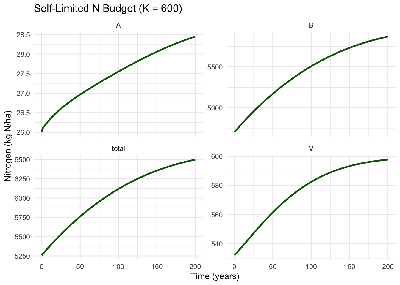
Figure 5.4: Dynamics of N budget with density-dependent vegetation growth. The system approaches equilibrium over ~150 years.
Interpretation:
Vegetation (V): Approaches K = 600 asymptotically. Growth is rapid initially, then slows as it approaches carrying capacity. After ~150 years, it’s essentially at equilibrium around 598 kg N ha⁻¹.
Available pool (A): Initially declines (same as before), but then slowly recovers as vegetation growth slows. At equilibrium, it stabilizes around 12-13 kg N ha⁻¹ - lower than the initial 26, but no longer being depleted.
Bound pool (B): Continues accumulating organic matter, but the rate slows as litter inputs slow (since V stops growing). Approaches equilibrium around 5,850 kg N ha⁻¹.
Total system: Continues accumulating because inputs > outputs, but the rate slows. The system is approaching a true steady state where inputs = outputs.
What causes equilibrium?
At equilibrium, dV/dt = 0, which requires either:
- V = 0 (trivial solution - no forest), or
- V = K (at carrying capacity), or
- a₁ × A = a₂ + a₃ (uptake rate equals loss rate)
In our model, the system approaches the third condition: V grows until it has drawn down A to a level where uptake exactly balances losses. The self-limitation ensures V can’t overshoot and oscillate.
5.15 Saving Your Model Function
Important for future work: Make a new R script containing just the bormann2 function. This creates a reusable module:
- Copy the complete
bormann2function definition - Paste it into a new R script
- Save as bormann2.R in your working directory
We’ll use this function in Chapter ?? for sensitivity analysis. Having it as a separate file makes it easy to source() into other scripts.
5.16 Common Issues and Troubleshooting
Here are solutions to problems students often encounter:
5.16.2 Warning: “lsoda– at t…, too much accuracy requested”
Cause: Usually indicates a parameter error making the system numerically unstable.
Troubleshooting steps: 1. Check that all parameters are positive (we took absolute values) 2. Verify units are consistent across all terms 3. Check for typos in the differential equation function 4. Make sure you’re subtracting losses, not adding them
5.16.3 Graph shows exponential explosion or negative values
Likely causes: - Sign error: adding a loss instead of subtracting, or vice versa - Missing absolute value: negative parameter causing growth instead of decay - Wrong units: parameter too large by a factor of 10, 100, etc.
Debug approach:
# Check parameter values
print(params)

# Run for just 1 year to see initial behavior
time_short <- 0:1
out_test <- ode(y = initial.state, times = time_short,
                func = bormann2, parms = params)
print(out_test)

# Calculate rates at initial conditions manually
with(as.list(c(initial.state, params)), {
  print(paste("dV/dt =", a1*A*V - a2*V - a3*V))
  print(paste("dA/dt =", i1 + a2*V + a4*B - a1*A*V - a5*A))
  print(paste("dB/dt =", i2 + a3*V - a4*B - a6*B))
})5.17 Connections to Previous Chapters
Let’s recap how this chapter builds on earlier material:
From Chapter 4: - We use the same balance equation framework: Change = Sources - Sinks - We verify mass balance by summing all compartments - We distinguish state variables (V, A, B) from parameters (a₁, a₂, etc.)
From Chapter 2: - We use constant (zero-order) inputs just like Example 1-4 - We see how constant inputs can lead to accumulation (Examples 1, 2) or depletion (Example 4)
From Chapter 3: - We use first-order loss kinetics: flux = k × Pool - We calculate steady states by setting dX/dt = 0 - We understand residence time and turnover - We see how coupling compartments creates interdependence
New in this chapter: - Combining zero-order and first-order processes in one model - Using literature data to estimate parameters - Distinguishing annual rates from instantaneous rates - Adding density-dependence (self-limitation) - Working with a real published ecosystem model
5.18 Summary and Key Takeaways
What you’ve learned:
Real ecosystems combine multiple rate types - some fluxes are constant (precipitation), others depend on pool sizes (mineralization, uptake)
Parameterization requires careful attention to:
- Units (always check that equations balance dimensionally)
- Signs (gains vs. losses)
- Rate types (instantaneous vs. annual)
Model interpretation is biological - don’t just make graphs, explain what they mean ecologically
Models iterate - we started simple (bormann1) and added realism (bormann2). This is normal!
Mass balance is non-negotiable - if total system change ≠ inputs - outputs, you have an error
Self-limitation is crucial for realistic long-term dynamics of biological populations and biomass
Next steps:
In Chapter ??, we’ll explore:
- How uncertainty in parameters affects predictions
- Which parameters matter most
- How to systematically explore parameter space
- Making robust predictions despite uncertainty
You now have a working ecosystem model based on real data. That’s a significant accomplishment!
5.19 References
Bormann, F.H., G.E. Likens, T.G. Siccama, R.S. Pierce, and J.S. Eaton. 1977. The export of nutrients and recovery of stable conditions following deforestation at Hubbard Brook. Ecological Monographs 47:255-277.
Soetaert, K. and P.M.J. Hermann. 2009. A Practical Guide to Ecological Modelling. Springer, Dordrecht.