7 NPZD - a simple aquatic ecosystem
The objective of this chapter is to understanding and explore a simple model of a nitrogen-limited aquatic ecosystem consisting of an inorganic pool, phytoplankton, zooplankton, and particulate detritus.
This Primer chapter relies entirely on selections in pages 31-58 of Soetaert and Herman (2009):
- 2.5-2.5.5: Functional responses and rate limitations.
- 2.6-2.6.2: Coupled model equations.
- 2.7.2: Closure.
- 2.8.2: Light, as a physical factor.
- 2.9.1: NPZD, a simple model of an aquatic ecosystem.
This background reading describes the anatomy of interactions. It builds on chapter 3 (Describing a nitrogen budget), and is critical for advancing your understanding of ecosystem compartment models.
One small piece of the background reading (sec. 2.5-2.5.5) concerns limitations and inhibitions on maximum fluxes. One of the most common ways to describe these limitations is closely related the Michaelis-Menten model originally proposed to describe enzyme kinetics (Fig. 7.1). There, the rate of change in a product, \(Y\), is a decelerating function of substrate concentration \(X\), \[\frac{dY}{dt} = V_m\frac{X}{k+X}\], where \(V_m\) is the maximum rate of change, and \(k\) is the half-saturation constant. The half-saturation constant is the value of the substrate \(X\) at which the rate is half the maximum, because it simplifies the expression to \(V_m\frac{X}{X+X} = \frac{1}{2}V_m\).
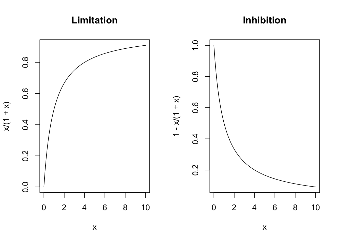
Figure 7.1: ‘Limitation’ arises when the benefit of a resource declines as the resource becomes super-abundant. ‘Inhibition’ is formulated as 1-limitation and arises when some factor such as a waste product or toxin increases in concentration.
7.1 This task
Below, I supply some code from Soetaert and Herman (2009). Your assignment is to make a copy of it, and document heavily it with your own comments. Nearly every line of code should have a comment. Use comments to demarcate different sections of the script. Don’t forget to start with comments about the what the document is, your name, and the source of the model.
Turn in your script, and the figure it should generate.
To begin, create or obtain an R script of the following code.
library(deSolve)

NPZD<-function(t,state,parameters)
 {
 with( as.list(c(state,parameters)), {
    PAR <- 0.5*(540+440*sin(2*pi*t/365-1.4))
    din            <- max(0,DIN)
    Nuptake <- maxUptake * PAR/(PAR+ksPAR) * din/(din+ksDIN)*PHYTO

    Grazing        <- maxGrazing * PHYTO/(PHYTO + ksGrazing)*ZOO
    Faeces         <- pFaeces * Grazing
    Excretion      <- excretionRate * ZOO
    Mortality      <- mortalityRate * ZOO * ZOO
    Mineralisation <- mineralisationRate * DETRITUS
    Chlorophyll    <- chlNratio * PHYTO
    TotalN         <- PHYTO + ZOO + DETRITUS + DIN

    dPHYTO    <- Nuptake - Grazing
    dZOO      <- Grazing - Faeces - Excretion - Mortality
    dDETRITUS <- Mortality - Mineralisation + Faeces
    dDIN      <- Mineralisation + Excretion - Nuptake


    list(
      c(dPHYTO,dZOO,dDETRITUS,dDIN),
      c(Chlorophyll = Chlorophyll, PAR=PAR, TotalN= TotalN)
      )
    })
  }

## THE FLUXES ARE PER DAYS. SCAlE PARAMETERS ACCORDINGLY.
parameters<-c(maxUptake          =1.0,       #
              ksPAR              =140,       #
              ksDIN              =0.5,       #
              maxGrazing         =1.0,       #
              ksGrazing          =1.0,       #
              pFaeces            =0.3,       #
              excretionRate      =0.1,       #
              mortalityRate      =0.4,       #
              mineralisationRate =0.1,       #
              chlNratio          =1)         #


state     <-c(PHYTO   =1,   #
              ZOO     =0.1,
              DETRITUS=5.0,
              DIN     =5.0)


times     <-c(0,365)
out       <- as.data.frame( ode(state,times, NPZD, parameters) )
out

num   <- length(out$PHYTO)   # last element

state <- c(PHYTO=out$PHYTO[num],
               ZOO=out$ZOO[num],
               DETRITUS=out$DETRITUS[num],
               DIN=out$DIN[num])

times     <-seq(0,730,by=1)
out <-as.data.frame(ode(state, times, NPZD, parameters))

out.long <- out %>% as.data.frame() %>%
  pivot_longer(-time, names_to="State_vars", values_to="Value")

ggplot(data=out.long, aes(time, Value)) +
  geom_line() +
  facet_wrap(~State_vars, scales="free_y")

## provide a unique name for your PNG file
ggsave("myNPZDplot.png")