11 More On Forcing Functions: Using data inside models
In previous chapters, we showed two ways of using external data as forcing functions. In NPZD - a simple aquatic ecosystem, we used seasonal variation in sunlight (PAR) using a mathematical expression in our R ODE function. In Multiple Element Limitation, we used the events argument to force a doubling of CO\(_2\) concentration. Here we demonstrate two methods (one new, one old) to use environmental data inside our system of ODEs using our model of a [terrestrial nitrogen budget]{#N#}. For our new method, we introduce the use of data interpolation, implemented in R using approxfun().
Our scientific goal in this chapter is to explain the decline in nitrogen export. This is happening in New England watersheds outside of Hubbard Brook, and it is not clear why.
11.1 Preliminaries
We’ll start by loading packages we need.
# rm( list = ls() ) # clean the workspace, with rm()
## load the libraries we need
## install these if you have not already done so.
library(tidyverse) # data management and graphing
library(deSolve) # ODE solver
Next, we load our own ODE function and parameters. Make sure you obtain an up to date copy of BormannLogistic.R.
## Make sure you obtain a new copy of BormannLogistic.R
source("code/BormannLogistic.R")
p <- c( I1 = 6.5, # deposition
        I2 = 14.2, # N fixation
        a1 = 79.6/(532*26), # uptake by vegetation (V)
        a2 = (6.6 + 0.8)/532, # root exudation into available pool
        a3 = (54.2 + 2.7 + 6.2 + 0.1)/532, # litter fall, etc.
        a4 = 69.6/4700, # net mineralization
        a5 = 3.9/26, # export from available pool to stream
        a6 = 0.1/4700, # export from bound pool to stream
        K = 600 # carrying capacity of vegetation
        )

## a02 0.0275559  0.0041165  6.6940 2.171e-11 ***
## a23 0.1434636
Finally, we’ll load environmental data. Note the trajectory of annual N export (kg/y, `ann.export.kg.y).
## we skip the first 7 lines because those contain metadata
HB.df <- read.csv("data/env_data_HB.csv", skip=7)
HB.df[1,]
## year factor value
## 1 1970 ann.exp.TN.kg.y 6.802761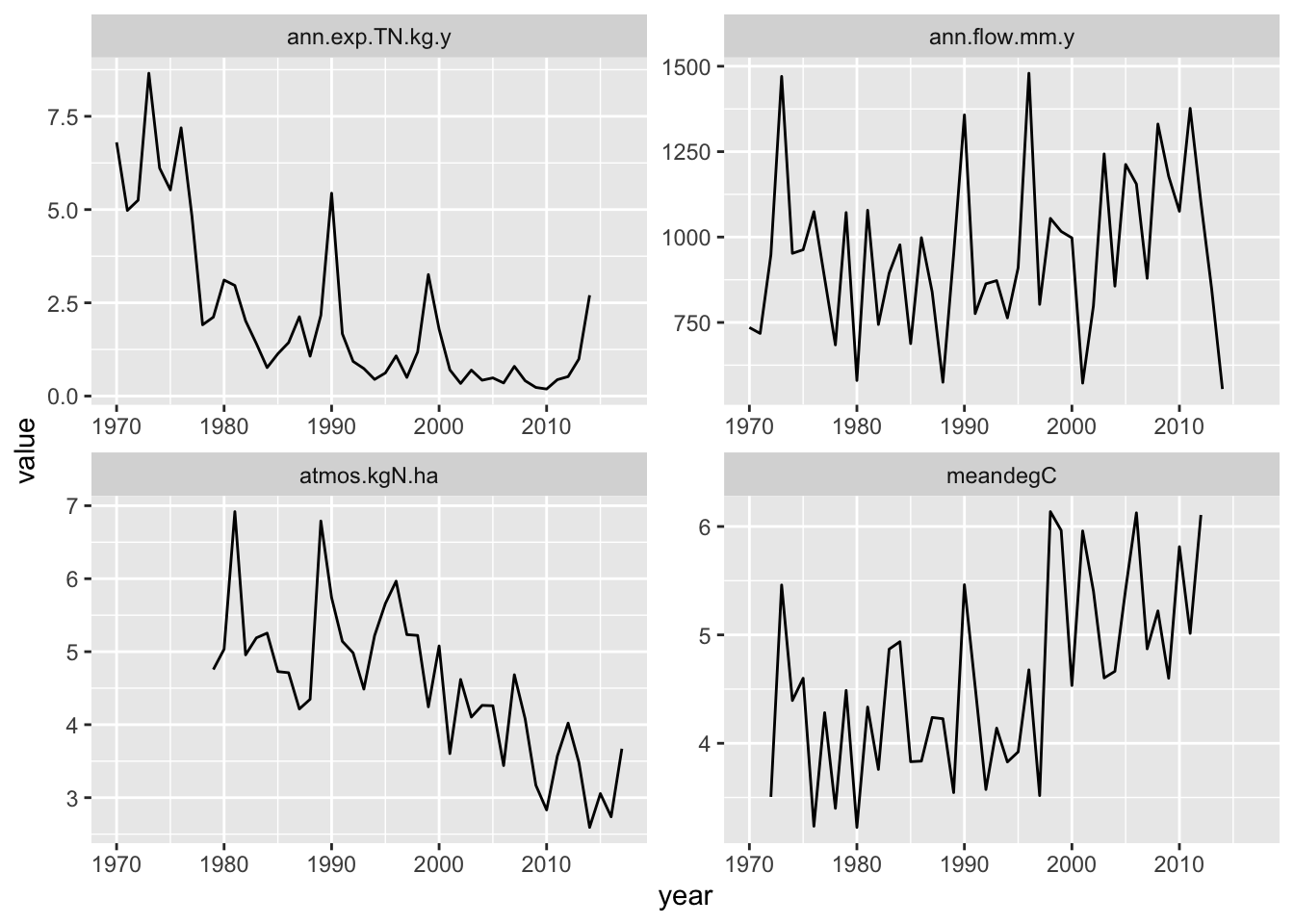
Figure 11.1: At the Hubbard Brook LTER, annual stream N export and N deposition have declined, while average annual temperature has increased. Average annual sream flow has been highly variable.
We see that average annual temperature has been increasing (meandegC) and N deposition has be decreasing. Could either of these be to blame?
11.2 N deposition
We see N deposition declining (Fig. 10.2), and so perhaps that is the most obvious answer to why stream export is declining. We will use these data to determine N deposition in our model (parameter \(I_1\)). This is an example of a “time-varying parameter”.
Creating a data-based time-varying parameter is not hard when we use interpolation. The reason we do this is because these data are only annual averages, but our ODE needs parameter values at potentially any instant in time. We will write a small function that will calculate a value for \(I_1\), based on surrounding data points.
Below, we use the following steps:
- Data wrangling, learning what years we have data for and creating a
timevariable. - Write a function to interpolate N deposition data between time points.
- Write code to update the model with N deposition.
- Generate model predictions and compare them visually to data, and to predictions from models without temperature.
We first need to extract the N deposition data, and create a new variable time instead of year that starts at zero instead of 1979.
## Find out the range of years for each state variable or factor
## Exclude missing data
HB.df %>% filter( !is.na(value)) %>%
  group_by(factor) %>% # group the data by state vars
  ## calculate stats (for each state var)
  summarize(first_year=min(year),
            last_year=max(year))
## # A tibble: 4 × 3
## factor first_year last_year
## <chr> <int> <int>
## 1 ann.exp.TN.kg.y 1970 2014
## 2 ann.flow.mm.y 1970 2014
## 3 atmos.kgN.ha 1979 2017
## 4 meandegC 1972 2012Here we select the data we want.
ndep <- HB.df %>% # select orig. data
  ##select non-missing deposition data only
  filter(!is.na(value) & factor== "atmos.kgN.ha") %>%
  ## add new variable t = 0,1, 2, .... max
  mutate( time = year - min(year) )
Next we use approxfun() to create the function to approximate N deposition for an arbitrary time point. We then plot the data and show the linear interpolation.
ndep.func <- approxfun(x = ndep[,"time"], y = ndep[,"value"], method = "linear", rule = 2)

## plot the data
plot(x = ndep[,"time"], y = ndep[,"value"],
     ylab="N deposition (kg/ha/y", xlab="Year (1979-2017)")
## add the linear interpolation
curve(ndep.func, 0, 38, add=TRUE, n=1001)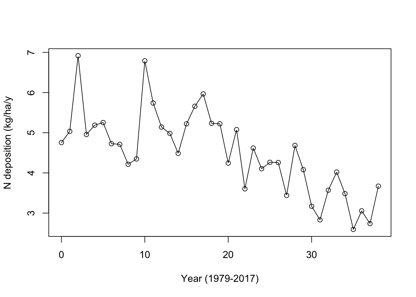
(#fig:lin_int)Linear interpolation between annual N deposition data points, using approxfun().
We can fit smoothed lines, splines, across these points as well. R allows a variety of methods for fitting splines, and here we show two.
## natural
ndep.func.nat <- splinefun(x = ndep[,"time"], y = ndep[,"value"], method = "natural")
## fmm: Forsythe, Malcolm and Moler (default)
ndep.func.fmm <- splinefun(x = ndep[,"time"], y = ndep[,"value"], method = "fmm")

## plot the data
plot(x = ndep[,"time"], y = ndep[,"value"],
     ylab="N deposition (kg/ha/y", xlab="Year (1979-2017)")
## add the smoothed interpolation
curve(ndep.func.fmm, 0, 38, add=TRUE, n=1001, lty=3, lwd=2)
curve(ndep.func.nat, 0, 38, add=TRUE, n=1001)
legend("topright", legend=c("Natural", "FMM"), lty=1:2, bty="n")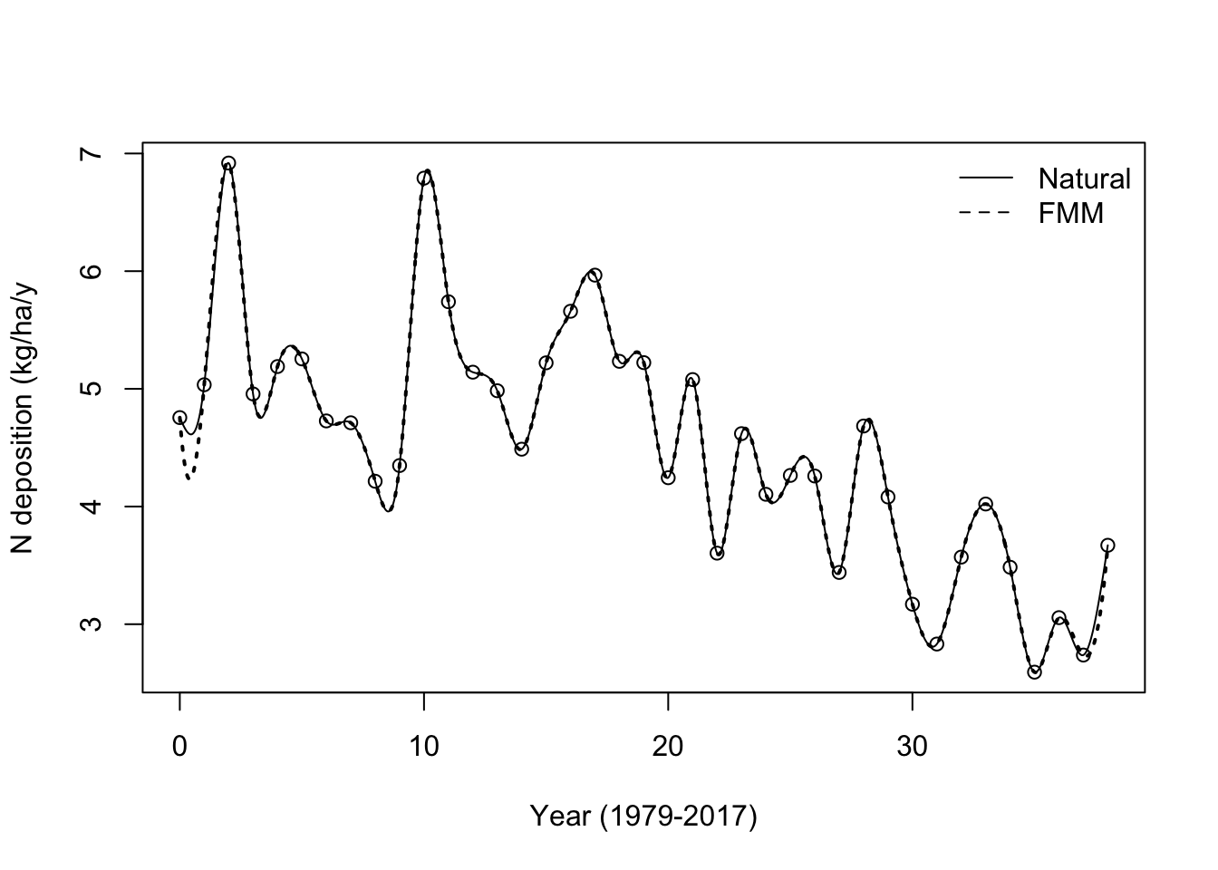
(#fig:spline_int)Smoothed interpolation between annual N deposition data points, using splinefun().
Next we write a new version of the ODE function that includes linear interpolation to create a new value of \(I_1\).
bormann.dep <- function(t, y, p) {
  with(as.list( c(y, p) ), {
    ### ODEs
    ## Rate of change = Gains - Losses
    ## I1 - deposition into the inorganic available pool
    ## I2 - N fixation
    ## a1 - plant uptake
    ## a2 - root exudate into the available pool
    ## a3 - litter fall
    ## a4 - mineralization
    ## a5 - is loss from Available to the stream
    ## a6 - is loss from the bound pool to the stream
    ##############
    ### Adding linearly interpolated N deposition
    I1.new <- ndep.func(t)
    ##############

    ## ODEs
    dV.dt <- (a1 * A * V  - a2 * V - a3 * V) * (1 - V/K )
    dA.dt <- ( I1.new + a4 * B ) - ( a1 * V * A + a5 * A)
    dB.dt <- I2 + a3 * V  - (a4 * B + a6 * B)

    ## loss from the soil to the stream and out the watershed
    export <- a5*A + a6*B

    # returning a list whose first  element
    # is a vector of the ODE values
    return(
      list(
        c( dV.dt, dA.dt, dB.dt ),
        export=export,
        I1.new=I1.new
           )
    )
    }
  )
}
Next we run the model, combine with our stream export data, and see what we get.
## This relies on the data set and functions we made above:
## ndep and ndep.func
## times that we want R to return
## just round years
t <- seq(from = 0, to = 38, by = 1)

y0 <- c(V = 532, A = 24, B = 4700)
## Integrate
out <- as.data.frame(
  ode(y = y0, times = t, func = bormann.dep, parms = p)
)

## combine with stream export data
exp.data <- HB.df %>%
  filter(year > 1978 & factor== "ann.exp.TN.kg.y")
out$export.data <- exp.data$value

## rearrange to long format, and reorder state variable levels
out2 <- out %>% as.data.frame() %>%
  pivot_longer(cols=V:export.data) %>%
  transform(name=factor(name, levels=c(
    "V", "I1.new", "export.data",
    "B", "A", "export") ) )

## plot
ggplot(out2, aes(time, value)) + geom_line() +
  facet_wrap(~ name, scales="free", nrow=2)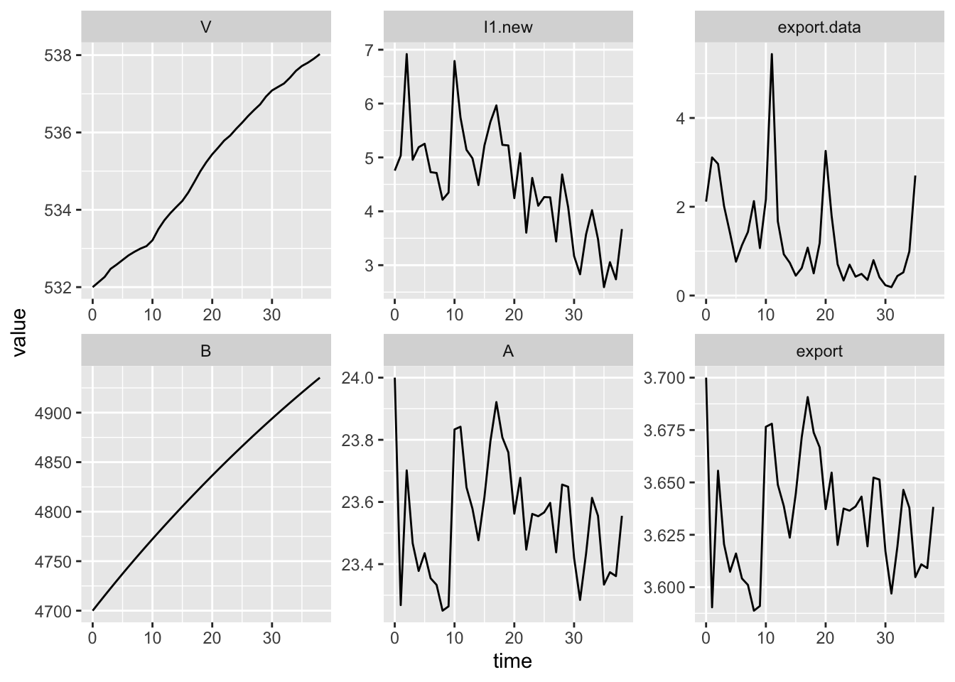
(#fig:ts.denitr)Declining deposition doesn’t guarantee declining export.
11.3 Denitrification
Denitrification will occur in both the forest floor and from the stream, wherever there is moisture, a lack of oxygen, and a source of nitrate (Chapin III, Matson, and Mooney 2011). All else being equal, denitrification rate increases with increasing nitrate. It might cause declines in stream export because this is measured at the bottom of the watershed. Unfortunately, our model does not currently include terms for denitrification. Lucky for us, we can add them.
Let’s model denitrification in both the forest floor and the stream as a first order process (\(aX\)). We will assume that denitrification causes loss from the forest floor, which is about 1/4 the total bound pool. GROFFMAN and TIEDJE (1989) found that well dranined Michigan forest soils lost 0.5–10 kg N/ha/y. If we take the midpoint of that range, we get 5 kg N/ha/y.
We’ll assume that denitrification occurs in the stream channel after leaching from the available pool. Mulholland et al. (2008) found that about 20% of nitrate entering reference watersheds was denitrified. This means the stream retains about 80% of the nitrogen that gets leached out of the soil and into the stream.
Here is a new version of our model, with both N deposition and dentrification.
bormann.denitr <- function(t, y, p) {

  with(as.list( c(y, p) ), {
    ### ODEs
    ## Growth = Gains - Losses
    ## I1 - deposition into the inorganic available pool
    ## I2 - N fixation
    ## a1 - plant uptake
    ## a2 - root exudate into the available pool
    ## a3 - litter fall
    ## a4 - mineralization
    ## a5 - is loss from Available to the stream
    ## a6 - is loss from the bound pool to the stream

    ### Adding N deposition
    I1.new <- ndep.func(t)

    ### Adding denitrification
    ## a7 is the mass-specific denitrification rate in the forest floor
    ## a8 is mass-specific denitrification from the stream
    ## Thus, (1-a8) is rate of N retention in the stream

    ## ODEs
    dV.dt <- (a1 * A * V  - a2 * V - a3 * V) * (1 - V/K )
    dA.dt <- ( I1.new + a4 * B ) - ( a1 * V * A + a5 * A)

    ## Adding denitrification from the forest floor
    ## param = a7 * (~1/4 of the bound pool)
    dB.dt <- ( I2 + a3 * V ) -  a4 * B - a6 * B - a7 * B/4

    ## loss from the soil to the stream
    leaching <- a5*A + a6*B

    ## export out of the watershed
    ## a8 is loss through dentrification
    export <- leaching - a8*leaching

    # returning a list whose first (and only) element
    # is a vector of the ODE values
    return(
      list(
        c( dV.dt, dA.dt, dB.dt ), I1.new=I1.new, export=export
           )
    )
    }
  )
}
Here we add denitrification parameters.
## Forest floor denitrification (Groffman et al. 1989)
## total rate / forest floor N
p["a7"] <- 5 / 1100

## Stream denitrification (Mulholland et al. 2008)
p["a8"] <- 0.2 #
Next we run the model, combine with our stream export data, and see what we get.
## This relies on the data set and functions we made above:
## ndep and ndep.func
## times that we want R to return
## just round years
t <- seq(from = 0, to = 38, by = 1)
y0 <- c(V = 532, A = 24, B = 4700)
## Integrate
out <- as.data.frame(
  ode(y = y0, times = t, func = bormann.denitr, parms = p)
)

## combine with stream export data
exp.data <- HB.df %>%
  filter(year > 1978 & factor== "ann.exp.TN.kg.y")
out$export.data <- exp.data$value
## rearrange to long format and plot
out2 <- out %>% as.data.frame() %>%
  pivot_longer(cols=V:export.data) %>%
  transform(name=factor(name, levels=c(
    "V", "I1.new", "export.data",
    "B", "A", "export") ) )

ggplot(out2, aes(time, value)) + geom_line() +
  facet_wrap(~ name, scales="free", nrow=2)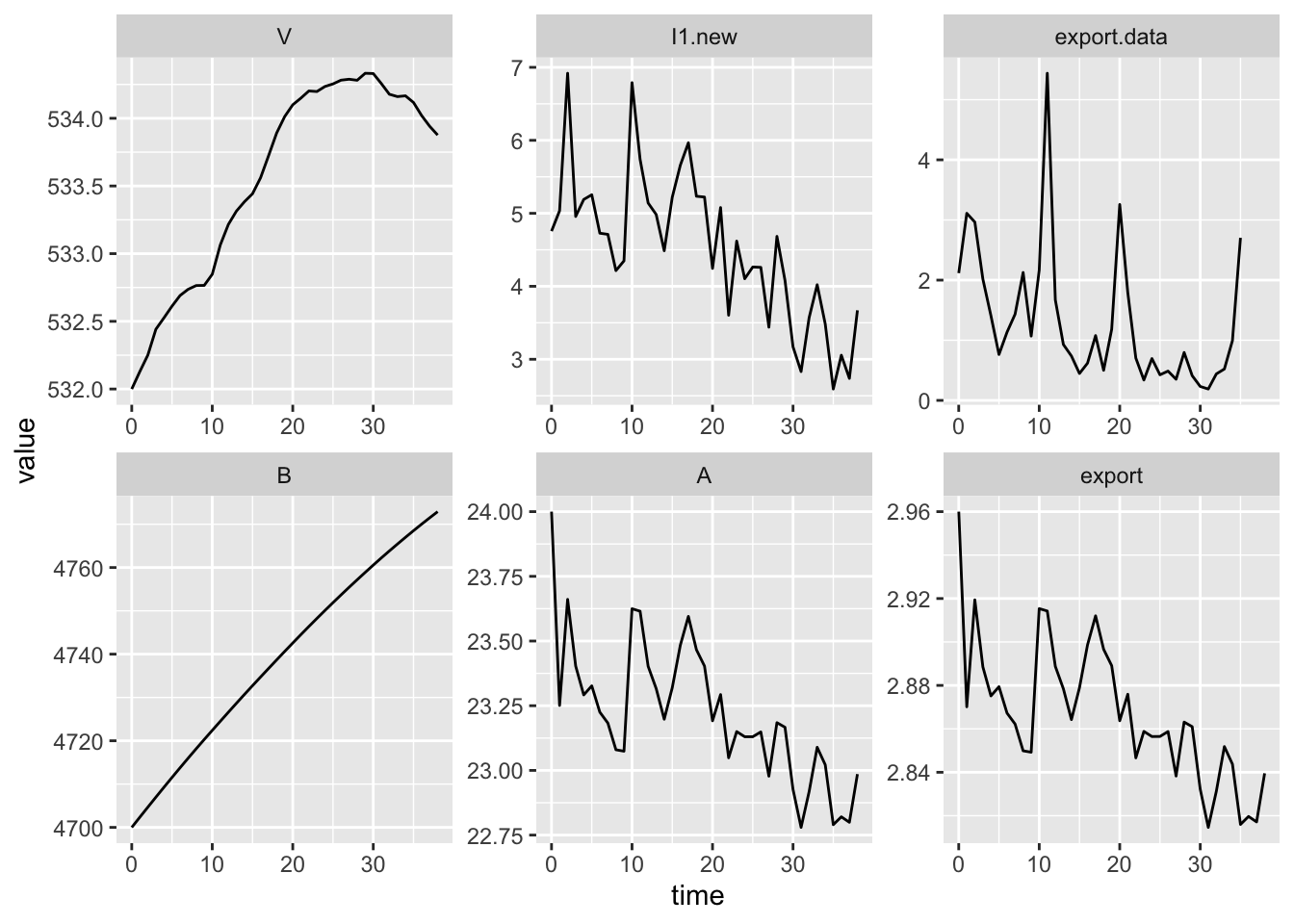
Figure 11.2: Dynamics with N deposition and denitrification in forest floor and stream.
11.4 Annual temperature as a forcing function
We see annual temperatures increasing so it is likely that these are influencing microbial processes associated with ecosystem flux. Increasing temperatures could be driving increases in mineralization, nitrification which could increase stream export if it is not taken up by plants or immobilized in microbial biomass. Increasing temperatures might increase denitrification rates, but like any of these, depends on precipitation as well.
Below, we use the following steps:
- Data management, making sure years align.
- Write code to update the model.
- Generate model predictions and compare them visually to data, and to predictions from models without temperature.
Here we use data on annual temperatures to scale selected rates using the \(Q_{10}\) relationship.
We first make sure that we are modeling years for which we have both N deposition and temperature data. We need to use the same years for temperatures as we did for N deposition, in our ndep data subset.
temps <- filter(HB.df, factor== "meandegC" &
                  !is.na(value) &
                  ## year *within* the ndep years
                  year %in% ndep$year) %>%
  mutate( time = year - 1979 )
## the min and max years in our data set
range(temps$year)
## [1] 1979 2012Next we can create the function to approximate N deposition for an arbitrary time point. We then plot the data and show the linear interpolation.
bormann.denitr.temp <- function(t, y, p) {

  with(as.list( c(y, p) ), {
    ### ODEs
    ## We hypothesize that the growth function is all that Bormann et al. included.
    ## Therefore, our logistic inhibition term acts on the entire forest.
    ## Growth = Gains - Losses
    ## Rate of change = Growth x Self-inhibition
    ## I1 - deposition into the inorganic available pool
    ## I2 - N fixation
    ## a1 - plant uptake
    ## a2 - root exudate into the available pool
    ## a3 - litter fall
    ## a4 - mineralization
    ## a5 - is loss from Available to the stream
    ## a6 - is loss from the bound pool to the stream

    ### Adding N deposition
    I1.new <- ndep.func(t)

    ### Adding denitrification
    ## a7 is the mass-specific denitrification rate in the forest floor
    ## a8 is mass-specific denitrification from the stream
    ## Thus, (1-a8) is rate of N retention in the stream

    ## Use temperatures
    ## interpolate to get instantaneous temperature
    inst.temp <- temp.func(t)

    ## create a temp multiplier using Q10 = 2 in parameters
    TempFactor <- exp( (inst.temp - ref.temp)/10 * log(Q10) )
    a4.new <- TempFactor * a4
    a7.new <- TempFactor * a7
    a8.new <- TempFactor * a8


    dV.dt <- (a1 * A * V  - a2 * V - a3 * V) * (1 - V/K )

    dA.dt <- ( I1.new + a4.new * B ) - ( a1 * V * A + a5 * A)

    dB.dt <- ( I2 + a3 * V ) -  a4.new * B - a6 * B - a7.new * B/4

    ## loss from the soil to the stream
    leaching <- a5*A + a6*B

    ## export out of the watershed
    export <- leaching - a8.new*leaching

    # returning a list whose first (and only) element
    # is a vector of the ODE values
    return(
      list(
        c( dV.dt, dA.dt, dB.dt ), I1.new=I1.new, export=export
           )
    )
    }
  )
}
Here we define \(Q_{10}\).
## This relies on the data set and functions we made above:
## temps and temp.func
## times that we want R to return
## just round years for the years in THIS data set
##
t <- seq(from = 0, to = nrow(temps)-1, by = 1)

p["ref.temp"] <- 3.5 # reference temperature from 1979
y0 <- c(V = 532, A = 24, B = 4700)
## Integrate
out <- as.data.frame(
  ode(y = y0, times = t, func = bormann.denitr.temp, parms = p)
)

## combine with stream export data
exp.data2 <- filter(exp.data, year %in% 1979:2012)
out$export.data <- exp.data2$value

## combine with temperature data
temp.data <- HB.df %>%
  filter(year %in% 1979:2012 &
           factor %in% "meandegC")
out$temp.data <- temp.data$value

## rearrange to long format and plot
out2 <- out %>% as.data.frame() %>%
  pivot_longer(cols=V:temp.data)

ggplot(out2, aes(time, value)) + geom_line() +
  facet_wrap(~ name, scales="free", ncol=3)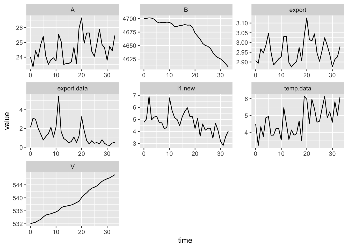
11.5 In fine
In this chapter, we described inclusion of forcing functions in an ODE model using interpolation. We did not yet answer the question of why stream N declines. One thing we did not do was explore the role of changing pool sizes. How would export respond to increasing pool sizes vs. stable pool sizes?