3 Simple Mass-specific Rates

This chapter concerns one and two compartment models with simple mass-specific fluxes.

3.1 Learning Objectives

• use simple 1- and 2-compartment models to track and predict fates of elements.
• use first order equations to represent inflows and outflows (fluxes) that are proportional to their source pool.
• calculate rates of change of mass in compartments, time to events, and make predictions about future states including steady states.

First-order kinetics

With first-order kinetics, the rate of a process is proportional to the amount of substrate present.

In a simple general form: \[\frac{dX}{dt} = \mathrm{Inputs} - k X\]

where \(k\) is the rate constant. The rate constant \(k\) represents a proportion of \(X\) at a given instant in time. Typically, we cannot say that it is a proportion of \(X\) across our entire time interval such as a day or a year, because \(X\) is usually changing over that time interval.

The units of \(k\) are “amount of \(X\) transferred per unit time per amount of \(X\) in the pool”, or

\[\mathrm{units}(k) = \frac{\mathrm{units}(X)}{\mathrm{units}(X)} \cdot \frac{1}{\mathrm{units}(t)}\] or, which simplifies to, \[\mathrm{units}(k) = \frac{1}{\mathrm{units}(t)}\]

For instance, imagine the rate water draining out of a bathtub per second is a function of the amount of the water in liters. The units of \(k\) would be “liters per liter per second” \[ \begin{align} \mathrm{units}(k) &= \frac{\mathrm{L}}{\mathrm{L} \cdot s}\\ &= \frac{1}{s} \end{align} \]

simplifying to just “per second”.

The fraction lost per unit time is constant, but the absolute amount lost decreases as the pool size declines.

3.2 Key Concepts

Read the following now, but apply them later as you work through the examples. Don’t sweat these too much to start. They will make more sense as you work through the examples.

1. STEADY STATE: At steady state for \(X\), \(X^*\), inputs = outputs
   • For first-order loss: \(\mathrm{Input} = kX^*\)
   • Therefore: \(X^* = \mathrm{Input}/k\)
2. MULTIPLE FIRST-ORDER LOSSES: Rate constants are additive
   • \(k_{\mathrm{total}} = k_1 + k_2 + k_3 + \ldots\)
3. RESIDENCE TIME: Average time a particle spends in the pool, at steady state,
   • \(\tau = X^*/\mathrm{Input} = 1/k_{\mathrm{total}}\)
   • Larger \(k_{\mathrm{total}}\) means faster turnover, shorter residence time
4. TURNOVER: At steady state, the proportion of the pool that gets replaced, or turns over, is \(k_{\mathrm{total}}\)
5. APPROACH TO STEADY STATE:
   • If \(X > X^*\): \(dX/dt < 0\) (pool declining toward steady state)
   • If \(X < X^*\): \(dX/dt > 0\) (pool growing toward steady state)
6. PARTITIONING LOSSES: At steady state, each pathway processes a fraction of the input proportional to its rate constant:
   • Fraction through pathway \(i = k_i/k_{\mathrm{total}}\)

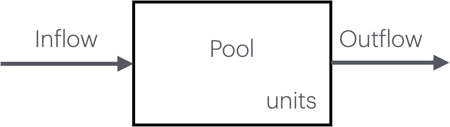
Figure 3.1: A one compartment model where Outflow is proportional to the pool.

For a one-compartment model of element \(X\) and first order kinetics, we can have one or more fluxes out. What is new is that those fluxes are functions of the size of the pool. So we still have the rate of change in the mass of \(X\) is \(\frac{dX}{dt} = F_{in} - F_{out}\), and now also where, \[F_{out} = kX\]

where flux units must match, for instance, \(\mathrm{units}(F_{in}) = \mathrm{units}(F_{out}) = \mathrm{kg\cdot y^{-1}}\), or kilograms per year, so units(\(k\)) = \(y^{-1}\) or \(1/y\)

3.3 Solving rate equations

Determining this steady state is Key Concept 1, above.

We often want to figure out whether a system is at an equilibrium or might achieve an equilibrium in the future. We call this equilibrium a steady state because the amounts in the pools remain “steady” or at constant amounts. That is, the state of the system remains constant, steady, unchanging. In other words, the rate of change, \(dX/dt\), is zero.

In general, we “solve” a rate equation by first setting it equal to zero, and then solving for \(X\) (the state variable):

\[ \begin{align*} \frac{dX}{dt} &= \mathrm{Inputs} - k X\\ 0 &= \mathrm{Inputs} - k X\\ k X &= \mathrm{Inputs}\\ X &= \frac{\mathrm{Inputs}}{k} \end{align*} \] What is this telling us?

It is telling us that the amount of \(X\) will stop changing when \(X\) reaches the amount predicted by the fraction \(\mathrm{Inputs}/k\).

You should work through the units on this to convince yourself the the units in each term are the same.

Solving a rate equation with constant rates is either simpler or less intuitive, depending on how you look at it. Essentially, when all the fluxes are constant, the only way we get a steady state is when the inflows are precisely equal to the outflows. Otherwise, a system with constant rates is predicted to forever increase or forever decrease, depending on the balance of inflows and outflows. If you walk through the arithematic we did above, you would find that the only way that the rate equation can equal zero is if the pool is empty (\(X=0\)) or \(F_{in}=F_{out}\).

3.4 One-compartment models

3.4.1 Worked Example: Lake phosphorus with flushing

A lake receives constant phosphorus input from a wastewater treatment plant but loses phosphorus proportional to the amount present due to water outflow.

• Constant input: \(I = 100\,\mathrm{kg\,P\,y^{-1}}\)
• First-order loss rate constant: \(k = 0.4\,\mathrm{y^{-1}}\)

The lake currently contains \(P = 300\,\mathrm{kg\,P}\).

Questions:

1. Draw a picture of the system.
2. Write the differential equation for \(dP/dt\).
3. Calculate \(dP/dt\) at the current phosphorus level4
4. Is the lake at steady state?
5. What phosphorus level would represent steady state? (‘Solve’ the differential equation)
6. Is the lake moving toward or away from steady state?

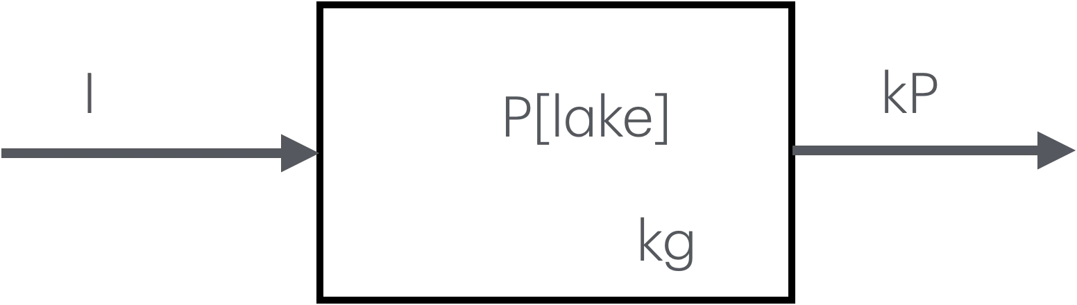
Figure 3.2: Picture of a one compartment model of phosphorus in a lake.

Differential equation \[\frac{dP}{dt} = I - kP\] where \(I = 100\,\mathrm{kg\,P/y}\), \(k=0.4\,\mathrm{y^{-1}}\), and the initial state is \(P_0 = 300\,\mathrm{kg\,P}\).

dP/dt at the current phosphorus level \[\frac{dP}{dt} = I - kP_0 = 100-0.4(300)= -20\, \mathrm{kg\,P\,y^{-1}}\]

Is the lake at steady state?

The lake \(P\) is not at steady state because the current rate of change (at \(P=300\)) is nonzero (negative,\(-20\, \mathrm{kg\,P\,y^{-1}}\).

To determine the amount of phosphorus that would be the steady state, or equilibrium, we solve \(dP/dt = 0\) for \(P\).

What phosphorus level would represent steady state?

To answer this question, we solve the differential equation (see above). We set it equal to zero because a value of zero means that the amount of phosphorus in the lake is not changing and so exists at a steady state.

By solving for \(P\), we are discovering the value of \(P\) when the system is at a steady state.

To determine the amount of phosphorus that would be the steady state, or the equilibrium, we solve \(dP/dt = 0\) for \(P\). Notice that the initial state doesn’t matter.

\[ \begin{align*} \frac{dP}{dt} &= I - kP\\ 0&= I - kP\\ kP &= I \\ P^* &= \frac{I}{k} = \frac{100}{0.4} = 250\,\mathrm{kg\,P} \end{align*} \] The star or asterisk on \(P^*\) signals that this is an equilibrium or steady state.

Is the lake moving toward or away from steady state?

Because the lake \(P\) is declining from 300 kg, it is moving toward it’s steady state.

3.5 Problems

3.5.1 Example 1: Watershed Nitrogen Loss

A forested watershed receives nitrogen through atmospheric deposition at a constant rate but loses nitrogen through leaching and stream export:

• Constant atmospheric deposition: \(I=7\,\mathrm{kg,N\,ha^{-1}\,y^{-1}}\)
• Leaching loss rate constant: \(k = 0.16\,\mathrm{y^{-1}}\)

The soil solution currently contains \(N=26\,\mathrm{kg\,N\,ha^{-1}}\).

Questions:

1. Draw a picture of the system.
2. Write the differential equation for \(dN/dt\).
3. Calculate \(dN/dt\) at the current nitrogen level.
4. Is the soil solution at steady state?
5. What nitrogen level would represent steady state?
6. Is the soil solution moving toward or away from steady state?

3.5.2 Example 2: Soil Organic Matter Decomposition

A soil layer receives organic matter from plant litter at a constant rate but decomposes following first-order kinetics.

• Constant litterfall input: \(I=500\,\mathrm{g\,C\,m^{-2}\,y^{-1}}\)
• Decomposition rate constant: \(k = 0.25\,y^{-1}\)

The soil currently contains \(C=1,800\,\mathrm{g\,C\,m^{-1}\).

Questions:

1. Write the differential equation for \(dC/dt\).
2. Calculate \(dC/dt\) at the current carbon level.
3. What is the steady-state carbon pool size?
4. How much carbon is being lost through decomposition right now?
5. At steady state, how much carbon would be lost per year through decomposition?

3.5.3 Example 3: Forest Canopy Nitrogen with Multiple Losses

A forest canopy receives nitrogen through atmospheric deposition at a constant rate but loses nitrogen through multiple first-order processes:

• Constant atmospheric deposition: \(I=8\, \mathrm{kg\,N\,ha^{-1}\,y^{-1}}\)
• Leaching loss rate constant: \(k_1 = 0.15\, \mathrm{y^{-1}}\)
• Herbivory loss rate constant: \(k_2 = 0.08\, \mathrm{y^{-1}}\)
• Litterfall rate constant: \(k_3 = 0.35\, \mathrm{y^{-1}}\)

The canopy currently contains \(N = 120\, \mathrm{kg\,N\,ha^{-1}\).

Questions:

1. Write the differential equation for \(dN/dt\).
2. What is the total loss rate constant (\(k_{\mathrm{total}}\))? See Key Concepts.
3. Calculate \(dN/dt\) at the current nitrogen level.
4. Calculate the steady-state nitrogen pool size.
5. At steady state, how much nitrogen is lost through each pathway annually?
6. What percentage of the canopy nitrogen pool turns over each year? Assume steady state.

3.5.4 Example 4: Stream Dissolved Organic Carbon

A stream reach receives dissolved organic carbon (DOC) from upstream at a constant rate, but processes it through multiple pathways:

• Upstream DOC input: \(I = 2,400\,\mathrm{g\,C\,d^{-1}}\)
• Microbial respiration rate constant: \(k_1 = 0.5\,\mathrm{d^{-1}}\).
• Photodegradation rate constant: \(k_2 = 0.2\,\mathrm{d^{-1}}\)
• Downstream export
  • Flow rate is \(Q = 10,000\,\mathrm{L\,d^^{-1}\)
  • Stream volume is \(V = 50,000\,\mathrm{L}\)
  • Export rate constant \(k_3 = Q/V\)

The stream currently contains \(C=6,000\,\mathrm{g\,C}\). In this problem, consider the carbon (\(C\)) in DOC only.

Questions:

1. Calculate the export rate constant \(k_3\).
2. Write the differential equation for \(dC/dt\) with all loss terms
3. What is the total loss rate constant?
4. Calculate \(dC/dt\) at the current DOC level
5. What is the steady-state DOC pool?
6. At steady state, how much carbon exits through each pathway daily?
7. What is the residence time of DOC in this stream reach at steady state? (See key concepts above.)

3.6 Two-compartment models

When we couple two compartments with first-order transfer, the rate of transfer between compartments is proportional to the amount in the source compartment.

General form for two compartments:

\[ \begin{align*} \frac{dN_1}{dt} &= F_{in} - k_{21}N_1 - k_{1,out}N_1\\ \frac{dN_2}{dt} &= k_{21}N_1 - k_{2,out}N_2 \end{align*} \]

where:

• \(k_{21}\) = rate constant for transfer into compartment 2 from compartment 1
• \(k_{1,out}\) = rate constant for loss from compartment 1 to outside
• \(k_{2,out}\) = rate constant for loss from compartment 2 to outside

Note that both rates have a shared term, \(k_{21}N_1\). This is an export from from one compartment and an import into the other, and its rate is proportional to the source.

At steady state: both \(dN_1/dt = 0\) AND \(dN_2/dt = 0\).

3.6.1 Key concepts for coupled compartments

Having connected or coupled compartments allows us to take advantage of several additional concepts.

1. COUPLED EQUATIONS: With first-order exchange, compartments are mathematically linked. Changes in one affect the other.
2. SOLVING FOR STEADY STATE:
   • Set both \(dN_1/dt = 0\) and \(dN_2/dt = 0\).
   • Solve the system of simultaneous equations.
   • Usually solve one equation for a ratio, then substitute.
3. BIDIRECTIONAL EXCHANGE: When compartments exchange material both ways, both differential equations include terms from the other compartment
4. MASS BALANCE CHECK: At steady state:
   • Total system input = total system output
   • Fluxes between compartments must balance; an export from one must be equal to imports into the others.
5. RESIDENCE TIME: More complex with exchange
   • Need to account for all inputs to a compartment
   • Including both external and internal (exchange) inputs
6. NET FLUX: With bidirectional exchange, calculate both directions then find net = larger flux - smaller flux
7. APPROACH TO STEADY STATE: Both compartments move toward their steady-state values, but at potentially different rates.

3.7 Answer Key

Example 1: Watershed Nitrogen Loss

1. A picture of the system.
2. \(dN/dt = I_D - kN\)
3. \(dN/dt = 7 - 0.16(26) = 2.84\)
4. The soil solution at steady state is not at steady state, but is increasing.
5. What nitrogen level would represent steady state?

\[ \begin{align*} \frac{dN}{dt} = 0 &= I_D - kN\\ kN &=I_D\\ N^* &= \frac{I_D}{k} = 7/0.16 = 43.75\,\mathrm{kg\,N\,ha^{-1}} \end{align*} \]

6. The soil solution is moving toward steady state.

Example 2: Soil Organic Matter

1. \(dC/dt = I - kC\)

2. \(dC/dt = 500 - 0.25(1,800) = 50\,\mathrm{g\,C\,m^{-2}\,y^{-1}}\)

   Soil carbon is accumulating (\(dC/dt>0\)).

3. At steady state: \[ \begin{align*} \frac{dC}{dt} = 0 &= 500 - 0.25C\\ C^* & = 500/0.25 = 2,000\,\mathrm{g\,C\,m^{-2}} \end{align*} \]

4. Current decomposition rate \(dC/dt = kC = 0.25(1,800) = 450 \,\mathrm{g\,C\,m^{-2}\,y^{-1}}\).

5. At steady state, output (decomposition) must equal input. Therefore, decomposition \(=500\, \mathrm{g\,C\,m^{-2}\,y^{-1}}\). We can check this also: 0.25 × 2,000 = 500.

Example 3: Forest Canopy Nitrogen

1. \(dN/dt = I - k_1N - k_2N - k_3N = 8 - (k_1 + k_2 + k_3)N\)
2. \(k_{\mathrm{total}} = 0.15 + 0.08 + 0.35 = 0.58\,y^{-1}\)
3. \(dN/dt = 8 - 0.58(120) = 8 - 69.6 = -61.6\,\mathrm{kg\,N\,ha^{-1}\,y^{-1}}\) The canopy is losing nitrogen
4. At steady state:

\[ \begin{align*} \frac{dN}{dt} = 0 &= I - (k_1 + k_2 + k_3)N\\ 0 &= 8 - 0.58N^*\\ N^* &= 8/0.58 = 13.8\,\mathrm{kg\,N\,ha^{-1}} \end{align*} \] e. At steady state (\(N^* = 13.8\,\mathrm{kg\,N\,ha^{-1}}\)): - Leaching: \(0.15(13.8) = 2.07\,\mathrm{kg\,N\,ha^{-1}\,y^{-1}}\) - Herbivory: \(0.08(13.8) = 1.10\,\mathrm{kg\,N\,ha^{-1}\,y^{-1}}\) - Litterfall: \(0.35(13.8) = 4.83 \,\mathrm{kg\,N\,ha^{-1}\,y^{-1}}\) - Total: \(2.07 + 1.10 + 4.83 = 8.0 \,\mathrm{kg\,N\,ha^{-1}\,y^{-1}}\,\checkmark\)

6. Turnover rate = \(k_{\mathrm{total}} = 0.58\,\mathrm{y^{-1}}\) = 58% per year.

Example 4: Stream DOC

1. \(k_3 = Q/V = 10,000/50,000 = 0.2\,\mathrm{d^{-1}}\)

2. \(dC/dt = I - k_1C - k_2C - k_3 C\)

3. \(k_{\mathrm{total}} = 0.5 + 0.2 + 0.2 = 0.9\,\mathrm{d^{-1}}\)

4. \(dC/dt = 2,400 - 0.9(6,000) = 2,400 - 5,400 = -3,000\mathrm{\,g\,C\,d^{-1}}\)

   Stream is losing DOC

5. At steady state:

\[ \begin{align*} \frac{dC}{dt} &= 2,400 - 0.9C\\ 0 &= 2,400 - 0.9C\\ C* &= 2400/0.9 = 2,667\,\mathrm{g\,C} \end{align*} \]

6. At steady state (\(\mathrm{C^* = 2667\,g\,C}\)):

   • Respiration: \(0.5 (2667) = 1,333 \,\mathrm{g\,C\,d^{-1}}\)
   • Photodegradation: \(0.2 (2667) = 533 \,\mathrm{g\,C\,d^{-1}}\)
   • Export: \(0.2 (2667) = 533 \,\mathrm{g\,C\,d^{-1}}\)
   • Total: \(1,333 + 533 + 533 = 2,400 \,\mathrm{g\,C\,d^{-1}}\)

7. Residence time: \(\tau = C^* / I = 2,667 / 2,400 = 1.11\,\mathrm{d}\)

   Alternative calculation: \(\tau = 1/k_{\mathrm{total}} = 1/0.9 = 1.11\,\mathrm{d}\)

   On average, a carbon atom spends 1.11 days in this stream reach.